Alternative Representation of Green’s Function for Electric Field
on Surfaces of Thin Vibrators
Yuriy M. Penkin, Victor A. Katrich, and Mikhail V. Nesterenko*
Abstract—An alternative representation of a Green’s function for electric fields on surfaces of thin impedance vibrators is proposed. The representation can be applied in software packages for simulation of RF and microwave devices. Advantages of the approach were demonstrated by analyzing the well-known problem of a thin symmetrical horizontal vibrator above a perfectly conducting plane. For a half-wave vibrator, numerical estimates of an effective external induced impedance were made for various distances between the vibrator and the plane. A possibility to realize a distribution of intrinsic impedance on the vibrator capable to compensate of the plane influence was also analyzed.
1. INTRODUCTION
Integral equations with Green’s function kernels are universal and effective tools of modern mathematical physics [1]. As well known, the Green’s function for a monochromatic vector field is an affinor, i.e., a symmetric tensor of the second rank. The affinor components are functions of mutual positions of two points: observation and source points, whose radius vectors are r andr, respectively. Apparently, the tensor Green’s functions in the theory of electrodynamics were considered for the first time in [2] and later were studied by many authors (e.g., [3–13]). Of course, numerical solutions of boundary value problems by integral equations can be conveniently obtained by using the Green’s functions, which operate on direct calculations of the electric field at the observation point.
Commercial software packages for simulation of microwave components are built on various mathematical methods [14], which can be classified into direct and indirect methods. The direct methods for solving boundary value problems include the finite element method (FEM) and finite difference time domain (FDTD) method. A characteristic feature of these methods is their versatility, allowing to simulate a large variety of complex microwave structures. The universality of the FEM and FDTD methods leads to substantial cost of computing resources and large computation time for the simulation of microwave structures, since the required number of discretization elements is usually very high. The FEM is used in the software package Ansoft HFSS [15], and the FDTD in combination with FEM is utilized in the CST Microwave Studio [16].
The indirect methods are an alternative to solution of the computational problems in electrodynamics. Among them, the method of moments (MoM) is the most suitable for the simulation of antenna system. This method differs from direct numerical approaches, since the field in observation point is found as an analytical solution of a certain key problem, namely, a problem of structures excitation by an elementary current source. This solution is uniquely determined by the Green’s function. The MoM approach is effective if the Green’s function can be represented analytically in a simple form. In this case, only a surface discretization is required, the dimensionality of the problem greatly reduces, and a full-wave 3D modeling of the microwave devices becomes possible. Unfortunately,
Received 26 October 2016, Accepted 29 November 2016, Scheduled 9 December 2016
* Corresponding author: Mikhail V. Nesterenko ([email protected]).
the Green’s functions can be simply found only for a limited number of structures, for example, for flat-layered media and the free space. Therefore, the MoM based CAD systems have been developed for simulation of these structures include: Microwave Office, ADS Momentum of Agilent [17], FEKO of EM Software & System [18]. Dyadic Green’s functions are also used in IE3D of Zeland Software system [19]. Thus, we can state that the further improvement of commercial simulation software is restricted by absence of a common methodological approach to presentation of the Green’s functions for volumes with compound boundaries. Therefore, the search and justification of such a methodological platform is a relevant and important problem for the engineering practice. We suppose that this approach to solution of vibrator problem can be implemented by utilizing a sourcewise presentation of the Green’s function (6), which allows us to make formalization of the same type in algorithms of the problem solution for volumes with boundaries of various geometries. The paper is aimed at development of a general procedure for the Green’s function representation (6) which can be used to define electric fields on surface of a thin impedance vibrator located in an arbitrary electrodynamic volume. Analysis of the term responsible for reaction of spatial domain boundaries is based on impedance concept [13, 20].
2. GENERAL TECHNIQUE FOR SOLVING THE VIBRATOR RADIATOR PROBLEM
If the monochromatic vector fields with the angular frequency ω depend on the time t as eiωt, the electrical Green’s functions of inhomogeneous vector equations, obtained from Maxwell’s equations, can be represented in a rectangular coordinate system as the solution of the following equations [13]
rotrot ˆGE(r, r)−k12GˆE(r, r) = 4πIδˆ (|r−r|), (1)
Δ ˆGA(r, r) +k21GˆA(r, r) = −4πIδˆ (|r−r|), (2)
which satisfy the boundary conditions of corresponding boundary value problem. Here, δ(|r−r|) = δ(x−x)δ(y−y)δ(z−z) is the three-dimensional Dirac delta function, ˆI = (ex⊗ex)+(ey⊗ey)+(ez⊗ez) is the unit tensor,ex,ey,ezare the unit vectors of the coordinate axes; Δ is the Laplace operator, symbol ⊗denotes the tensor product, k1 =k√ε1μ1, k= 2π/λ is the wave number,λis the wavelength in free
space, and (ε1, μ1) are the permittivity and permeability of the medium. The tensor ˆGE(r, r) is called
by the Green’s function for the electric field, and ˆGA(r, r) is the Green’s function for the vector potential in accordance with the applicable version of the equation.
The Green’s function allows us to derive a closed form expression for electromagnetic fields of arbitrary vector sources at any point in space. If the source is given by an electric current density
Je(r) in the volume V, the electric field can be represented by following expressions:
E(r) = k
2 1
iωε1
V ˆ
GEr, rJerdr, (3)
E(r) = 1 iωε1
graddiv +k12
V ˆ
GAr, rJerdr, (4)
The difference between formulas (3) and (4) can formally be associated with different calibrations of the electromagnetic field potentials. For an infinite homogeneous medium, the only boundary condition imposed on the Green’s function is the Sommerfeld’s radiation condition. For example, the Green’s function for the vector potential obtained as the Equation (2) solution can be represented as
ˆ
GA(r, r) = ˆIe
−ik1|r−r|
|r−r| . (5)
Ifr=r, the Green’s functions ˆGE(r, r) and ˆGA(r, r) for any spatial domain go to infinity, and the integrals in Eqs. (3), (4) cannot be defined as the Riemann sums [13]. However, it is possible to understand the integrals in the Cauchy principal value sense, isolating a singular part in the Green’s function for the vector potential [1, 13]:
ˆ
GAr, r= ˆIGr, r+ ˆGV0A
whereG(r, r) =e−ik1|r−r|/|r−r|, and ˆGV
0A(r, r) is a regular function which satisfies the homogeneous
equation
Δ ˆGV0A
r, r+k12GˆV0A
r, r= 0 (7)
and satisfies the boundary condition on the surfaceS of the volumeV for the field point source, located at the point r. The representation of the Green’s function in Eq. (6) is called by the sourcewise representable.
Let us consider the integral equation [20] for the current on the surfaceSof an impedance vibrator. The equation is valid for any electrodynamic volume filled with an isotropic homogeneous medium can be written as
1 iωε1
(graddiv +k21)
S ˆ
GA(r, r)J(r)dr =−E0(r) +zi(r)J(r), (8)
whereJ(r) is the electric current on the vibrator;zi(r) is the linear intrinsic impedance of the vibrator ([Ohm/m]); E0(r) is the field of extraneous source. Substituting the sourcewise representation of the
Green’s function in Equation (6) in Equation (8), we obtain the following equation
1 iωε1
(graddiv +k21)
S
ˆ Ie
−ik1|r−r|
|r−r| + ˆG V 0A r, r
J(r)dr =−E0(r) +zi(r)J(r). (9)
Let us consider the linear impedance vibrator represented by a segment of a circular cylinder whose radius is r and length 2L. If inequalities 2rL 1 and r
√ε 1μ1
λ 1 hold, the thin-wire approximation allows us to reduce Eq. (9) to an equation with quasi-one-dimensional kernel [20, 21]
S
ˆ Ie
−ik1|r−r|
|r−r| + ˆG V 0A r, r
J(r)dr ≈ L
−L J(s)
e−ik1√(s−s)2+r2
(s−s)2+r2 + ˆG
V
0A
s, s ds, (10)
wheres, s are local coordinates related to the vibrator axis. Both terms of the integrand are continuous functions at any point on the vibrator generatrix. Therefore, the differentiation operators can be transferred to the integral, and Equation (10) can be written as
L
−L J(s)
∂2 ∂s2
e−ik1√(s−s)2+r2
(s−s)2+r2
+k21
e−ik1√(s−s)2+r2
(s−s)2+r2 ds
+
⎛
⎝graddiv +k12
L
−L
J(s)es·GˆV0A
r, es·sds, es
⎞
⎠−zi(s)iωε1J(s) =−iωε1E0(s), (11)
wherees is the unit vector directed along the axis of the vibrator.
The first term in the left-hand side of Equation (11) coincides with that of the well-known Pocklington’s equation [22] for a perfectly conducting vibrator in the free space. This equation is interpreted as the vibrator self-field which can be rewritten in the form proposed by Richmond [23]
L
−L J(s)
∂2 ∂s2 +k
2 1
e−ik1R
R ds
=
L
−L J(s)e
−ik1R
R5
(1+ik1R)
2R2−3r2+k12r2R2
R=√(s−s)2+r2
ds. (12)
The second term in Eq. (11) is the functional which takes into account the response of the electrodynamic volume boundary to the vibrator current. This term also needs a correct physical interpretation. The authors of this article have proved a general theorem [24], stating that the influence of the volume boundaries on the current of a perfectly conducting radiator can be compensated by coating the vibrator by the complex impedancezi(s). In our notation, this impedance should satisfy the identity
zi(s) = −i ωε1J(s)
⎛
⎝graddiv +k21
L
−L
J(s)es·GˆV0A
r, es·sds, es
⎞
In accordance with physical similitude principle, one can assert that the physical analysis of the functional related to the boundary influence should be carried out in terms of the impedance concept. That is, to analyze the influence of the borders on the intrinsic vibrator characteristics, one must introduce the concept of the external effective induced impedance
ze(s) = ωε i
1J(s)
⎛
⎝graddiv +k21
L
−L
J(s)es·GˆV0A
r, es·sds, es
⎞
⎠. (14)
As it follows from the theorem, the requirements for the compensation of the boundary response are reduced to the equality zi(s) =−ze(s). The external induced impedance should be defined as effective impedance, since in a general sense, the condition Reze(s) ≥ 0 cannot be fulfilled. This condition is imposed by energy considerations which define the intrinsic impedance of the vibrator as a true physical quantity. However, the introduction of the effective impedance ze(s) is methodologically appropriate, since it allows us to localize the influencing factor of the external scattering surfaces on the vibrator radiators already at the level of the initial equation.
Thus, Equation (11) can be represented as
1 iωε1
L
−L J(s)e
−ik1R
R5
(1+ik1R)
2R2−3r2+k21r2R2
R=√(s−s)2+r2
ds−[ze(s) +zi(s)]J(s) =−E0(s).
(15) Comparing Equations (15) and (3), we can write the Green’s function for the electric field on the surface of a thin impedance vibrator
GEs, s= e
−ik1R
k21R5
(1 +ik1R)
2R2−3r2+k12r2R2
R=√(s−s)2+r2
−iωε1
k12
[ze(s) +zi(s)]δ(s−s),
(16) whereδ(s−s) is the Dirac delta function.
Expression (16) has a number of methodological features. First, the self-field generated by the vibrator currents and the secondary fields defined by boundaries of the electrodynamic volume and by the intrinsic vibrator impedance are combined by the simple relation. This allows us to calculate these terms by using various methods. Secondly, the representation of the boundary reaction in the form of the effective induced impedance ze(s) makes possible to use the identical formalization of computational algorithms for areas with boundaries of different geometry. Thirdly, using the first theorem proved in [24], we can easily justify the possibility to solve Equation (11) by the method of successive approximations, in which the secondary fields in Eq. (16) are determined using the vibrator current determined in the previous approximation. The above properties show that the Green’s function in Eq. (16) can be successfully used in commercial software packages to enhance their functionality.
One should bear in mind that the Green’s function in Eq. (16) was obtained using a mathematical formalism based on the quasi-one dimensional kernel in the integral Equation (9), therefore the simulation results will be approximate to a certain extent. This should be taken into account when numerical methods for the integral equation solution and their realization are selected (see, e.g., [25, 26]). One may also understand that the errors defined by the kernel approximation and excitation model by a concentrated load cannot always be separated. Although the analysis of these issues is beyond the scope of this paper, we can state that if the analytical methods of the integral Equation (9) solution are used, the simulation results for exact and approximate equations kernel are practically identical [27]. We will use this property in the next section.
3. FIELD OF A VIBRATOR ABOVE AN INFINITE PLANE
The boundary value problem for the thin symmetrical horizontal vibrator radiating in the uniformly filled half-space above the perfectly conducting half-plane is a classic problem of the modern electrodynamics theory. During the last hundred years, the problem for perfectly conducting and impedance vibrators was repeatedly studied by various authors (see, e.g., [11, 20, 21, 23, 26, 28–32]). In the thin wire approximation, the quasi-one dimensional kernel can be used, and the initial equation for the problem solution can be written in the following form
S ˆ
Ge(r, r)J(r)dr ≈ L
−L J(s)
e−ik1√(s−s)2+r2
(s−s)2+r2 −
e−ik1√(s−s)2+(2h+r)2
(s−s)2+ (2h+r)2 ds
, (17)
where h is the distance between the vibrator axis and the plane. The second term in the integrand of relation (17) can be interpreted as the Green’s function component associated with the vibrator mirror image in the perfectly conducting plane. Historically, this approach has been adopted as the most common. As a result, the influence of the plane on the vibrator radiation is usually interpreted in terms of intrinsic and mutual resistances of the vibrator and its mirror image. In other words, the physical processes of the vibrator radiation were interpreted using the functional quantities which emerge during the problem solution, but did not appeared in formulation of the initial problem. The mathematical results obtained by using this approach are quite correct, but, from the physical point of view, they look like a methodological casus. The fact is not only that the physical processes are interpreted as non-existing quantities, but such an interpretation cannot be generalized to other cases, e.g., for the impedance plane or for boundary surfaces of compound geometries. The proposed impedance interpretation which takes in account the influence of the extraneous scatterers on the radiating vibrator is free of these shortcomings. In this section, we will consider the numerical estimation of the effective induced impedanceze(s) for different distances between the vibrator and the plane. We will also analyze a possibility to select the intrinsic impedancezi(s), which can compensate the plane influence.
The problem geometry and adopted notations are shown in Fig. 1, where{x, y, z}is the Cartesian coordinate system and the axissis directed along the vibrator. As the initial equation for the problem
solution, we will use the Equation (11) in the form
d2 ds2 +k
2 1
L
−L
J(s)e
−ik1R(s,s)
R(s, s) ds
= −iωε1E0S(s) +
d2 ds2 +k
2 1
L
−L
J(s) e
−ik1√(s−s)2+(2h+r)2
(s−s)2+ (2h+r)2ds
+iωε
1zi(s)J(s), (18)
which allows us to obtained the explicit expression for the effective induced impedance of the vibrator located in the half-space above the plane as
ze(s) =− i ωJ(s)
d2 ds2 +k
2
L
−L
J(s) e
−ik√(s−s)2+(2h+r)2
(s−s)2+ (2h+r)2 ds
. (19)
If the vibrator in the infinite free space is exited in the center by a lumped voltage generator with an amplitudeV0, the current on the vibrator can be obtained as the solution of the corresponding problem
by the averaging method [13, 20] and can be written as
J(s) =−αV0
ik 60
sink(L− |s|) +αPδs(kr, ks)
coskL+αPLs(kr, kL) . (20)
Here α = 2 ln[r/1(2L)],Pδs(kr, ks) =Ps[kr, k(L+s)]−(sinks+ sink|s|)PLs(kr, kL), Ps[kr, k(L+s)] and PLs(kr, kL) are defined by the formulas, which were obtained in an explicit form in [13, 20]
Ps[kr, k(L+s)] = s
−L
e−ikR(s,−L) R(s,−L) +
e−ikR(s,L)
R(s, L) sink(s−s
)ds
s=L
= e ikL 2i L −L
e−ikR(s,−L)
R(s,−L) +
e−ikR(s,L)
R(s, L) e
−iks
ds
−e−ikL 2i
L
−L
e−ikR(s,−L) R(s,−L) +
e−ikR(s,L) R(s, L) e
iks
ds,
PLs(kr, kL) =
2 ln 2−γ(L)−Cin(4kL) +iSi(4kL) 2
coskL+Si(4kL)−iCin(4kL)
2 sinkL,
where Si(x) and Cin(x) are the sine and cosine integral functions of complex arguments, and
γ(s) = ln[(L+s) +
(L+s)2+r2] [(L−s) +(L−s)2+r2]
4L2 .
Let us substitute the expression for the vibrator current of Eq. (20) in Eq. (19), and change the order of integration and differentiation. Then, the final expression for the effective induced impedance along the vibrator axis can be presented as follows
ze(s) =− 30i kF i(s)
L
−L
F isF es, sds, (21)
whereF e(s, s) = e(−ikRR 1(s,s)
1(s,s))4 [
(s−s)2(3ik−Rk12(−s,s3))−R1(s, s)
−ik(R1(s, s))2+k2(R1(s, s))3
],F i(s) = sink(L− |s|) +αPδs(kr, ks),
R1(s, s) =
The numerical calculations for half-wave vibrator (2L = 0.5λ, r = L/100) have shown that the distribution of the effective induced impedance in Eq. (21) along a vibrator for h ≥ λ is U-shaped. Fig. 2 shows the plots of the effective complex impedance of one vibrator arm, Ze(s) = ze(s)/(120π), normalized by the resistance of free space. The curves were plotted for the three fixed distances. The U-shaped distribution is really expectable, since the denominator at the right-hand side of expression (19) contains the current distribution satisfying the boundary conditions J(±L) = 0. That is, distribution Ze(s) has singularities at the vibrator edges. However, theze(s) appears in formula (15) as the product ze(s)J(s), which at the edges of the vibrator is zero. Therefore, the valuesze(±L) were replaced by the approximate valuesze(±L)≈ze(±L∓r/2) [23].
As can be seen from Fig. 2, the flat curve segments in the plots of the real ReZe(s) and imaginary ImZe(s) parts of the complex impedance become expanded and more uniform when the distance between the vibrator and plane is increased. The values of ReZe(s) and ImZe(s) are decreased and at distances (h ≥ λ, h → ∞) become infinitesimal, since the plane has no significant effect on the vibrator in the points that are far from the vibrator ends. A more complete explanation of the plane influence on the
Figure 2. The distribution of the effective impedance along the vibrator arm: 2L = 0.5λ, r=L/100; 1−h= 1.25λ, 2−h= 2λ, 3−h= 20λ).
(a) (b)
(c) (d)
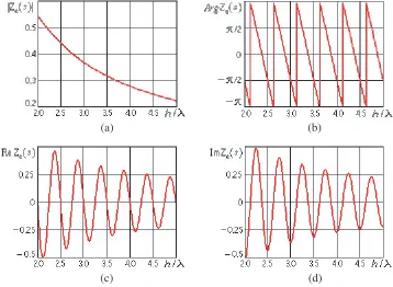
effective impedance induced on the vibrator can be derived by analyzing Fig. 3 which shows theZe(h/λ) plots obtained at the points s=L/2 in the middle of the vibrator arm.
As expected, the modulus of the effective impedance|Ze(L/2)|is characterized by an exponentially decaying dependence on h/λ and its argument is represented by the sawtooth periodic function with a period equal to λ/2 varying in the range [−π;π]. Accordingly, ReZe(s) and ImZe(s) are periodic oscillatory functions with decreasing amplitude (Fig. 3(c) and Fig. 3(d)). These functions are out of phase, therefore the effective impedance in the vicinity of points h = nλ/2, n = 1,2,3, . . . is of imaginary character, and its real part is close to zero. In the vicinity of pointsh=nλ/4,n= 1,3,5, . . . the impedance is of the real character, and the imaginary part is close to zero. In the second case, a resonant radiating vibrator remains resonant, but its radiating capacity is defined by the real part of the effective impedance. Since the impedance ReZe(s) can take both positive and negative values, the vibrator radiation resistance can be both increased and decreased.
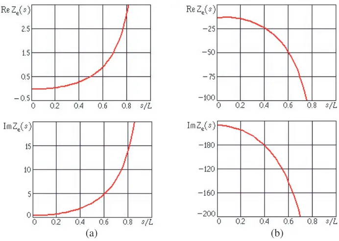
At distances 0≤h≤1.5λ, the plane causes rapid variation of ReZe(s) and ImZe(s) which can be up to several hundreds of times greater than the resistance of the free space (Fig. 4).
(a) (b)
Figure 4. The distribution of the effective impedance along the vibrator arm: 2L = 0.5λ, r=L/100; (a)h= 0.5λ, (b)h= 0.25λ.
Under these circumstances, the numeric estimate of the induced impedance variation using its value in a local point on the vibrator is impossible. The similar trends can be also observed at short distances h. The pointsh1 ≈0.356λand h2 ≈0.61λare characteristic, since ImZe(s) reverses its sign
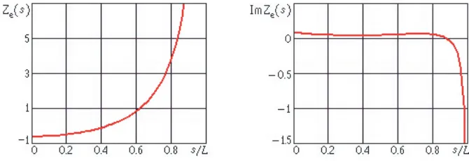
in these points. The plots of the effective induced impedance for h2 ≈ 0.61λ is shown in Fig. 5. As
is well known, the first two theoretically predicted resonances are experimentally observed just at the distancesh1 ≈0.356λ andh2 ≈0.61λ[20, 30]. We have also observed that the calculated impedance is
Figure 5. The distribution of the effective impedance along the vibrator arm: 2L = 0.5λ, r=L/100, h= 0.61λ.
The technological issues are related to difficulties in manufacturing vibrators with predefined profile of the intrinsic impedance [20]. The vibrators with the constant intrinsic impedance are most simple from the technological point of view. Therefore, a question concerning usage of the vibrators with the constant impedance for compensation the plane influence is aroused. One solution of the problem
consists in comparison of the two integral functionals: J1 =
L
−LF i
2(s)ze(s)ds and J 2 =zc
L
−LF i
2(s)ds,
where zc is the constant impedance of the vibrator. The functional J1 describes the influence of the
plane on the vibrator; it can be found in solution of Equation (18) obtained by the generalized method of the induced electromotive forces (EMF) [20]. The functionalJ2, is an asymptotic formula for functional
J1 if thezcvalue is correctly selected. Numerical simulations have shown that for the half-wave vibrator
an acceptable value of the constant impedance should be selected as
zc = Re (ze(0.05λ)) +iIm (ze(0.115λ)). (22) Although the above representation of the effective impedance is not optimal in the sense of mathematical strictness, its usage is acceptable for the distances h ≥ 2λ as can be seen from the Table 1. One can also notice thatJ1 andJ2 coincide at large distances. Thus, we can state that the influence of the plane
on the perfectly conducting vibrator at distances h ≥ 2λ can be compensated by using the relation zi(s) =−zc if the impedancezc is defined by the formula (22). At shorter distances the compensation should be done only by using the identityzi(s) =−ze(s).
Table 1. Dependences of the functionals J1 and J2 on the distance from the plane.
h 2.25λ 2.5λ 5λ 10.25λ 20λ
J1 −0.206 +i1.819 0.195−i1.641 0.117−i0.822 −0.062 +i0.401 0.033−i0.205
J2 −0.232 +i1.821 0.215−i1.642 0.122−i0.823 −0.063 +i0.401 0.033−i0.205
The effective induced impedance in Eq. (21) is inherently frequency dependent, but the estimates obtained above for a fixed wavelength can be used to analyze the vibrator radiation in an operating waveband. The data obtained for the middle of the vibrator waveband are valid for the whole wavelength range. The numerical simulation has shown that the real part of the vibrator effective impedance changes in a minor way (see Fig. 6), and its (imaginary practically part does) imaginary part practically does not change if the vibrator length is varied in the range 0.23λ≤L≤0.25λ.
4. CONCLUSION
The paper proposes a new representation of the Green’s function for the electric field on the surface of thin impedance vibrator. We suppose that the representation may be used in commercial software packages to enhance their functionality. The representation of the reaction of electrodynamic volume boundaries on the vibrator in the form of external effective induced impedance is the important feature of the new approach. The approach allows us to use one universal algorithm for volumes with boundaries of various geometry.
The advantages of the proposed approach were demonstrated by solving the radiation problem of thin symmetrical horizontal vibrator above a perfectly conducting plane. The dependences of the induced effective impedance upon the distance between the vibrator and the plane were obtained for the half wavelength vibrator. It was found that the distribution of the effective impedance along the vibrator is U-shaped. In the pointL/2 on the vibrator, the modulus of the effective impedance|Ze(L/2)| is exponentially decaying function of h/λ, while its argument ArgZe(L/2) is the sawtooth periodic function with the range of values [−π;π] and period equal toλ/2. At distances 0≤h≤1.5λ, the plane influence causes rapid variation in distributions of real and imaginary parts of the effective impedance along the vibrator, its value can be up to several hundreds of times greater than the resistance of the free space. On the basis of the theorem [24], the possibility to compensate the influence of the external plane by applying the intrinsic impedance to the vibrator surface was investigated. At distancesh≥2λ, the influence can be compensated by using the vibrators, characterized by the constant impedance distribution.
REFERENCES
1. Khizhnyak, N. A., Integral Equations of Macroscopical Electrodynamics, Naukova dumka, Kiev, 1986 (in Russian).
2. Levin, H. and J. Schwinger, “On the theory of electromagnetic wave diffraction by an aperture in an infinite plane conducting screen,”Commun. Pure Appl. Math., 355–391, 1950.
3. Morse, P. M. and H. Feshbach, Methods of Theoretical Physics, McGraw-Hill, New York, 1953. 4. Collin, R. E.,Field Theory of Guided Waves, McGraw-Hill, New York, 1960.
5. Van Bladel, J., “Some remarks on Green’s dyadic for infinite space,” IRE Trans. Antennas and Propagat., Vol. 9, 563–566, 1961.
6. Markov, G. T. and B. A. Panchenko, “Tensor Green functions of rectangular waveguides and resonators,”Izvestiya Vuzov, Radiotechnika, Vol. 7, 34–41, 1964 (in Russian).
7. Tai, C. T.,Dyadic Green’s Function in Electromagnetic Theory, Intex Educ. Publ., Scranton, 1971. 8. Tikhonov, A. N. and A. A. Samarsky, Equations of Mathematical Physics, Nauka, Moscow, 1977
(in Russian).
9. Felsen, L. B. and N. Marcuvitz,Radiation and Scattering of Waves, Prentice-Hall, Inc., New Jersey, 1973.
10. Penkin, Yu. M. and V. A. Katrich, Excitation of Electromagnetic Waves in the Volumes with Coordinate Boundaries, Fakt, Kharkov, 2003 (in Russian).
12. Nesterenko, M. V., D. Yu. Penkin, V. A. Katrich, and V. M. Dakhov, “Equation solution for the current in radial impedance monopole on the perfectly conducting sphere,” Progress In Electromagnetics Research B, Vol. 19, 95–114, 2010.
13. Nesterenko, M. V., “Analytical methods in the theory of thin impedance vibrators,” Progress In Electromagnetics Research B, Vol. 21, 299–328, 2010.
14. Vasylchenko A., Y. Schols, W. De Raedt, and G. A. E. Vandenbosch, “A benchmarking of six software packages for full-wave analysis of microstrip antennas,” Proceeding of the 2nd European Conference on Antennas and Propagation, EuCAP’2007, Edinburgh, UK, Nov. 11–16, 2007. 15. Ansoft Corporation, HFSS v. 10.1.1 User Manual, Jul. 2006, http://www.ansoft.com. 16. CST GmbH., CST Microwave Studio v. 2006B, www.cts.com.
17. Agilent Technologies, EEsof EDA, Momentum, http://eesof.tm.agilent.com/products/ momen-tum main.html.
18. EMSS — EM Software & Systems Ltd, FEKO Suite 5.2 User Manual, Jan. 2006, http: Hwww.emss.co.za.
19. Zeland Software, Inc., IE3D v. 11.2 User Manual, Jan. 2006, http: Hwww.zeland.com.
20. Nesterenko, M. V., V. A. Katrich, Yu. M. Penkin, V. M. Dakhov, and S. L. Berdnik,Thin Impedance Vibrators. Theory and Applications, Springer Science+Business Media, New York, 2011.
21. King, R. W. P., The Theory of Linear Antennas, Harv. Univ. Press, Cambr., MA, 1956.
22. Pocklington, H. C., “Electrical oscillations in wires,” Proc. Cambr. Phil. Soc., Vol. 9, Pt. VII, 324–332, 1897.
23. Mittra, R.,Computer Techniques for Electromagnetics, Pergamon, New York, 1973.
24. Penkin, Yu. M., V. A. Katrich, and M. V. Nesterenko, “Development of fundamental theory of thin impedance vibrators,” Progress In Electromagnetics Research M, Vol. 45, 185–193, 2016.
25. Fikioris, G. and T. T. Wu, “On the application of numerical methods to Hallen’s equation,”IEEE Trans. Antennas Propagat., Vol. 49, 383–392, 2001.
26. King, R. W. P., G. Fikioris, and R. B. Mack, Cylindrical Antennas and Arrays, Cambridge University Press, Cambridge, UK, 2002.
27. King, R. W. P., E. A. Aronson, and C. W. Harrison, “Determination of the admittance and effective length of cylindrical antennas,” Radio Science, Vol. 1, No. 7, 835–850, 1966.
28. Sommerfeld, L., “Uber die ausbereitung electromagnetisher wellen in der jdrahtlosen telegrafie,”
Annalen der Physik, Vol. 28, 665, 1919.
29. Markov, G. T., and D. M. Sazonov, Antennas, Energiya, Moscow, 1975 (in Russian). 30. Eisenberg, H., “Short-wave antenna,” Radio and Svyaz, Moscow, 1985 (in Russian).
31. Feinberg, E. L., Propagation of Radio Waves over the Earth Surface, Nauka, Moscow, 1999 (in Russian).