Analysis Challenges for High Dimensional Data

(1)

Western University Western University

Scholarship@Western

Electronic Thesis and Dissertation Repository

4-27-2018 10:30 AM

Analysis Challenges for High Dimensional Data

Bangxin Zhao

The University of Western Ontario

Supervisor He, Wenqing

The University of Western Ontario

Graduate Program in Statistics and Actuarial Sciences

A thesis submitted in partial fulfillment of the requirements for the degree in Doctor of Philosophy

Follow this and additional works at: https://ir.lib.uwo.ca/etd

Part of the Applied Statistics Commons, Biostatistics Commons, Microarrays Commons, Multivariate Analysis Commons, Numerical Analysis and Scientific Computing Commons, Statistical Methodology Commons, and the Theory and Algorithms Commons

Recommended Citation Recommended Citation

Zhao, Bangxin, "Analysis Challenges for High Dimensional Data" (2018). Electronic Thesis and Dissertation Repository. 5370.

https://ir.lib.uwo.ca/etd/5370

This Dissertation/Thesis is brought to you for free and open access by Scholarship@Western. It has been accepted for inclusion in Electronic Thesis and Dissertation Repository by an authorized administrator of

(2)

Abstract

The practical and theoretical challenges posed by the ‘largep, smalln’ settings are

important issues in contemporary statistics. In this thesis, we propose new

methodolo-gies that target three diﬀerent areas of high-dimensional statistics: variable screening,

inﬂuence measure and post-selection inference.

Variable screening is a general procedure in high dimensional data analysis to

en-sure the applicability of statistical methods. Typically marginal correlation between

the response and each predictor are employed for this role. It is a complicated and

computationally burdensome procedure since spurious correlations commonly exist

among predictor variables, and important predictor variables may not have large

marginal correlations with the response variable. We propose a new estimator for

the correlation between the response and high-dimensional predictor variables, and

based on the estimator we develop a new screening technique termed Dynamic

Tilt-ed Current Correlation Screening (DTCCS) for high dimensional variables screening.

DTCCS is capable of picking up the relevant predictor variables within a ﬁnite number

of steps. The DTCCS method includes the widely used sure independence screening

(SIS) method and the high-dimensional ordinary least squares projection (HOLP)

approach as special cases. The DTCCS technique has sure screening and

consisten-cy properties which are demonstrated theoretically and numerically and illustrated

through a real-life example.

Two methods of high-dimensional inﬂuence measure have also been explored.

They are from the perspective of the extreme value distribution (EVD) and the

robust-ness of design respectively. For the ﬁrst method, EVD-type statistics have been shown

to be powerful in measuring high-dimensional inﬂuence theoretically and numerically.

From the second method, we propose Hellinger distance for high-dimensional

inﬂu-ence measure (HD-HIM). The inner product of two transformed inﬂuence functions

is used to measure the Hellinger distance of two discrete distribution functions from

(3)

that have unusual eﬀect on high-dimensional models. The HD-HIM method has been

illustrated theoretically and numerically.

Lastly, we propose a post-selection inference method termed Cosine PoSI that is

numerically feasible in a high-dimensional framework. Cosine PoSI focus on the

geo-metric aspect ofLeast Angle Regression (LARS). LARS eﬃciently provides a solution

path along which the entered predictors always have the same absolute correlation

with the current residual. At each step of the LARS algorithm, the proposed Cosine

PoSI method employs an angle from the correlation between the entering variable

and current residual and considers this angle as a random variable from the cosine

distribution. The post-selection inference is then conducted based on the order

statis-tics of this cosine distribution. Given the collection of the possible angles, hypothesis

tests are performed on the limiting distribution of the maximum angle. To conﬁrm

the eﬀectiveness of the proposed method, we conduct simulation studies and a real-life

data analysis to illustrate the usefulness of this post-selection method.

KEYWORDS: High-dimensional statistics, variable screening, deterministic

(4)

Acknowledgements

This dissertation could not have been possible without the help and the support of

several individuals. First and foremost, I would like to express my deepest gratitude

to my beloved supervisor, Dr. Wenqing He, for his immense support and extremely

valuable guidance throughout my Ph.D. study. Without his consistent and

illuminat-ing instruction, I would not be where I am today. I not only learned new statistical

knowledge from him, but also learned how to conduct research with creativeness and

better vision. His enthusiasm to help his students will always be a good example and

guide me in my future.

I would also like to express my heartfelt gratitude to the examiners of my thesis

defense committee, Dr. John Koval, Dr. Jiandong Ren, Dr. Douglas Woolford and

Dr. Mu Zhu, for their time, insightful questions, valuable comments, suggestions and

discussions on my research work. I want to thank Dr. Reg Kulperger for sharing his

vast knowledge and giving suggestions during my thesis and proposal writing.

I owe my honest gratitude to Dr. David R. Bellhouse, Dr. Ian McLeod, Dr. Serge

Provost, Dr. Hao Yu and Dr. Ricardas Zitikis. I also want to thank all the faculty

members and staﬀ in our department for their invaluable help. Their kindness and

help during these wonderful years at the University of Western Ontario is appreciated.

Many special thanks go in particular to Dr. Grace Y. Yi for sharing her valuable

experience in scientiﬁc writing and paper preparation.

I want to thank Dr. Wenqing He again, and Dr. Rohana J. Karunamuni, Dr.

Qingguo Tang for being great co-authors.

I am deeply grateful for all the fun time I had with my friends during my Ph.D.

study. I thank Xin Liu, Jiang Wu, Wenjun Jiang for being great oﬃcemates and for all

the interesting discussions and sports time. I appreciate all the cultural discussions

and game play with Wisdom Stallone Avusuglo and Hossein Zareamoghaddam. I

thank Dexen Xi, Chen Yang, Guandong Zhang, Kexin Luo for the R discussions. It is the dream of everyone to play an important role on the stage surrounded

by loyal audiences. However, our sense of security, hopefulness, conﬁdence, and

(5)

midst of despondency, insecurity, and disappointment. I consider myself a lucky fellow

to have such supportive family members. Especially, my wife, Zhe (Aggie) Yu, and my

parents whose unwavering support and love these years cannot be overemphasized. I

(6)

List of Tables

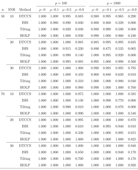
2.1 Screening Accuracy for Scenario I . . . 48

2.2 Screening Accuracy for Scenario II . . . 50

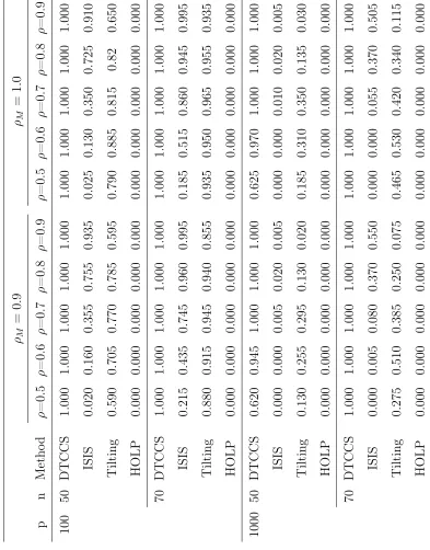
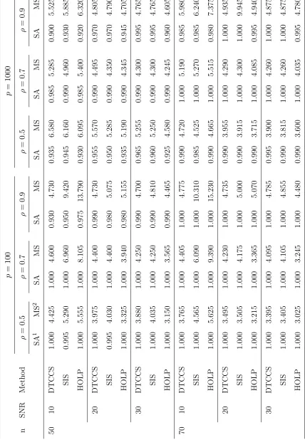
2.3 Screening Accuracy and Final Model Size for Scenario III . . . 52

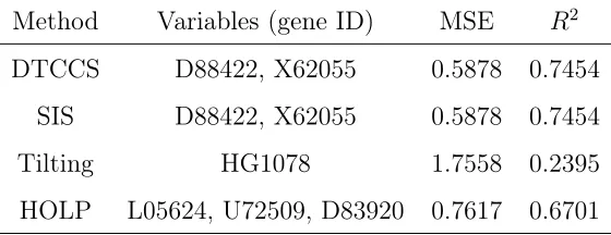
2.4 Data Analysis of Leukemia Data (LOOCV) . . . 54

2.5 Final Models for Leukemia Full Data using Diﬀerent Methods . . . . 54

3.1 Inﬂuence Detection of EVD-HIM . . . 90

3.2 Simulation results for case 1 withK = 1 . . . 92

3.10 Simulation results for case 2 with K = 4 . . . 101

(10)

4.1 Selected Model Size and Selection Accuracy for Scenario I . . . 122

4.2 Selected Model Size and Selection Accuracy for Scenario II . . . 123

4.3 Data Analysis of Eye Microarray Data (LOOCV) . . . 125

(11)

List of Figures

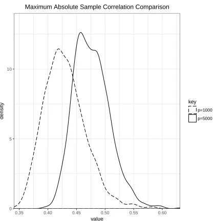
1.1 Distribution of the maximum absolute sample correlation coeﬃcients

between X1 and {Xj}j̸=1 when n = 60; p = 1000 (dashed curve) and

n= 60; p= 5000 (solid curve). . . 14

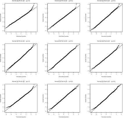
2.1 Normal QQ Plot for β/τ with ρ= 0.1, . . . ,0.9. . . 68

3.1 Power comparison between HIM and HD-HIM of case 1 . . . 97

(12)

Chapter 1 Introduction

1.1 Motivation and Purpose of the Dissertation

With rapid development in technologies, a growing number of research ﬁelds

en-counter data with unprecedented size and complexity, such as researches in artiﬁcial

intelligence, economy, ﬁnance, biology, genetics, engineering and astronomy. The

importance of data and the vitality of data analysis cannot be downplayed in

con-temporary science. As computational power increases and the expense of data

collec-tion and processing decrease signiﬁcantly, the dimension of datasets is continuously

becoming large. In those dataset, the dimension of predictor variables p can be as large as or much larger than the sample size n, but very often, among thousands of available predictor variables only a small number of them are informative and it is

critically important to identify them correctly. High-dimensional data analysis has

re-ceived a tremendous of attention recently. Seminal theories ofLeast Angle Regression

(LARS, Efron et al. 2004) and Sure Independence Screening (SIS, Fan and Lv 2008)

both proposed to use correlation between predictor variables and response (or current

residual) to solve high-dimensional problems. The high-dimensional correlation can

be viewed as a counterpart to ordinary least square (OLS) estimator of the parameter

and many data-driven methods based on correlation have been studied for years in

high dimensional statistics. In this dissertation, we develop new methodologies and

(13)

The methodologies proposed in this dissertation is aiming to solve but not limited to

the following high-dimensional problems:

Example 1.1.1. Hastie et al. (2009): Microarrays gene expression data

Microarrays gene expression data is one of the classical high-dimensional data

types. DNA microarrays measure the expression of a gene in a cell by measuring the

amount of mRNA present for that gene. A gene expression data set collects together

the expression values from a sequence of DNA microarray experiments, with each

column representing an experiment. There are therefore several thousand (p) rows

representing individual genes and tens (n) of columns representing samples.

Typical questions about microarray data: certain genes show abnormal expression

for certain cancer sample; certain genes are more important in a certain disease and

et cetera. Traditional statistical methods can not be directly applied to answer those

questions.

Example 1.1.2. Biba and Xhafa (2011): High-dimensional text regression

The design matrix of the bag-of-words (BOW) model consists rows of high

dimen-sional vector whose elements are the frequency of words. The BOW model has been

widely applied in machine learning topics such as email ﬁltering. For more details

see Biba and Xhafa (2011). Statistical diagnostic techniques can be also contribute

to these problems. We measure the inﬂuence of the high-dimensional observations

(the email) and expect to automatically ﬂag the email category and give warning to

a suspicious email.

Besides the above two examples, other high-dimensional problems to which the

methods developed in this thesis could be applied are image recognition (pixels of the

high resolution images are large); spatial correlation of home prices (up to 1 million

spatial parameters), retailer real-time pricing (for millions of items), amongst others.

In the rest of this chapter, we provide a review of the literature on the relevant

topics covered in this thesis, which include matrices with applications in statistics,

development in high-dimensional sparse modelling and estimation, robust statistics

(14)

1.2 The High-dimensional Design Matrix

Over the past decade, advancement of new technologies in the ﬁelds of the natural and

social sciences have improved data collection procedures. This has led to the problem

of high-dimensional data analysis which links to the idea of a complicated large design

matrix, denoted X. For this n×pdesign matrix, the number of predictor variables, p, is either on the same order of, or much greater than, the number of observations, n. For instance, data ascertained from spectra, biomedical imaging, high-frequency ﬁnance and DNA micro-arrays can be of high-dimension. The traditional methods

that perform well for low-dimensional data run into many severe problems in analyzing

such a dimensional dataset. The common issues that arise in analyzing a

high-dimensional dataset by using traditional methods include: the non-invertibility of the

matrix XTX, the high correlation among predictors in the model, the non-existence

of the inverse covariance matrix (precision matrix), amongst others.

The high-dimensional dataset with p≈n or p > ncan be divided into two cases:

high dimension and ultra-high dimension. If the dimensionalitypgrows polynomially with the sample sizen, i.e.,p=O(nα)for someα >0, we call ithigh dimension; if the dimensionality p grows non-polynomially with the sample size n, i.e., p=O(enι

) for someι ∈(0,1), we call itultra-high dimensionornon-polynomial (NP) dimensionality

(Fan and Lv 2008; Shao and Deng 2012).

We begin with the most important and commonly used regression model, the

classical linear regression model. Linear regression model investigates the

relation-ship between a continuous dependent variable (normally referred to as the response

variable), and at least one explanatory variable (also known as predictor or

covari-ate). In classical statistical model setting, the number of observations is typically

denoted asn, while the number of predictors in a model (referred to as the dimension of the model) is denoted as p. For subject i in a sample of n individuals, let yi be

the response variable and xi = (xi1, xi2, . . . , xip)T be the p dimensional predictors.

(15)

and X=

       

xT

1 xT₂ .. .

xT_n

       

be the n×p design matrix including thepdimensional predictors

for n subjects. In this thesis, the subset columns or rows of the design matrix are frequently used. X˜₋j denotes the submatrix of deleting the jth predictor variable,

Xj, j = 1, . . . , p. X(−i) denotes the submatrix of deleting the ith observation, xi,

i = 1, . . . , n. To ease the notations, we use Xj, j = 1, . . . , p, for the jth predictor

variable and the its realization in the design matrix. The relationship between the

response y and the predictor variables (X1, . . . ,Xp)T is given by

y=β1X1+β2X2+· · ·+βpXp+ϵ, (1.1)

where ϵ is the random error. Alternatively, this classical model can be written with realization in sample size n,

Y =Xβ+ϵ, (1.2) where β ∈Rp is the vector of the coeﬃcients and ϵ∈Rn is the noise term. Usually,

we assume ϵ ∼ N(0, σ2_I₎_{. Alternatively,} _X _{can be considered as a row of column} vectors: X = (X1,X2,· · · ,Xp), where Xj = (x1j, . . . , xnj)T for j = 1, . . . , p. Let

row(X) be the linear p−dimensional space which is spanned by the row vectors of X and col(X) be the linear n−dimensional space which is spanned by the column vectors of X.

Now, let xbe ap dimensional random vector with multivariate distribution with mean µp×1 and covariance Σp×p deﬁned as follows:

E(x) =µ, cov(x) = Σ.

(16)

Let ¯xand S denote the sample mean and sample covariance matrix, respectively. Deﬁne1n = (1, . . . ,1)T, an n×1 vector of ones, so that we have

¯

x= 1

nX

T₁

n (1.3)

and

S = 1

n(X−X¯)

T₍_X₋_X_¯₎_, _(1.4)

whereX¯ is an×pmatrix with each row comprised ofx¯T. It must be noted here that

¯

x and S are unbiased and consistent estimators forµandΣrespectively. The sample covariance matrix S is a good estimator of the population variance if n ≫ p, but it performs poorly when p is close to or larger than n (Cai et al. 2016). In the high-dimensional context, the estimation of the precision matrix (Ω = Σ−1, the inverse of the covariance matrix) is also a diﬃcult and computational complex question.

Cai et al. (2011) proposedconstrainedl1−minimization for inverse matrix estimation

(CLIME) to directly calculate Ω by an optimization problem

min∥Ω∥1 subject to|SΩ−Ip|∞ ≤λn, (1.5)

where ∥ · ∥1 is the elementwise L1 norm (∥Ω∥1 =

∑

i,j|Ωi,j|), ∥ · ∥∞ is the matrix

elementwise inﬁnity norm (∥Ω∥∞= max

1≤i,j≤p|Ωi,j|), andλn= clog(p)

n for some suﬃciently

large constant c. This method has been built in the R packageclime, but it is still a time-consuming computing process to obtain the estimated precision matrix in

high-dimensional statistics.

In the random design setting for linear regression, each pair (xT_i ,yi)is the

obser-vation sampled from the population, where random vector xi = (xi1, . . . , xip)T ∈ Rp

and random variable yi ∈ R1. If the design matrix X in Eq. (1.2) consists of

random vectors, we call X a random design matrix. The random xi’s are usually

assumed to be independent identically distributed (i.i.d.) and independent of ϵi’s,

and βˆ= [cov\(xi)]−1cov\(xi,yi).

The ﬁxed design setting is the opposite of the random design setting, and the

design matrix in this setting is called deterministic design matrix. Let X˜₋j be the

(17)

orthogonal complement of the column space of X˜₋j. By using a deterministic design

matrix, the least square estimator can be expressed as βˆj = (X⊥j T

Y)/(X⊥_j TXj)for a

linear model without intercept, whereX⊥_jTXj ̸= 0forn > p(Zhang and Zhang 2014).

These two settings of the design matrix bring two views of parameter estimation:

a probabilistic one and a nonprobabilistic one. The goal of both views is to ﬁnd

coeﬃcients βˆsuch that the expected prediction error on a new observation from the

population is small enough. For the past two decades, statisticians extended those two

views to high-dimensional data, and developed many contemporary methodologies

and techniques for large random or deterministic design matrix, see details in Fan

and Lv (2008), Shao and Deng (2012), Lv (2013), Zhang and Zhang (2014) and

Wang and Leng (2016).

The column space (also called the range or image) of a design matrix X is

com-monly used in parameter estimation in the case ofn > p. The ordinary least squares (OLS) estimate projects the responseY onto the linear spacecol(X)which is spanned by columns of X. Due to lack of suﬃcient degrees of freedom, OLS is no longer

fea-sible for high-dimensional statistics. This motivates the idea of variable screening,

i.e., to obtain a subset of features that have signiﬁcant impact on the response before

building a formal statistical model. In contrast with column space ofX, row space of

X has been studied recently under high-dimensional setting. Shao and Deng (2012)

proposes an approach to project the parameter vectorβonto the linear spacerow(X)

which is spanned by the rows ofXand show that this projection ofβcan discriminate

large and small elements eﬃciently by choosing a proper thresholding value.

For p > n, considering the ridge regression estimator of β (Hoerl and Kennard 1970) under model (1.2),

ˆ

β_ridge = (XTX+λIp)−1XTY, (1.6)

where λ > 0 is an appropriately chosen regularization parameter. Shao and Deng (2012) and Wang and Leng (2016) show that the computation of βˆ_ridge involves only

inverting ann×n matrix since(XT_X₊_λI

p)−1XT =XT(XXT+λIn)−1 which implies

(18)

1.3 High-dimensional Linear Regression

1.3.1 Penalized Regression

Due to rapid development of technological advances, modern scientiﬁc research very

often encounters datasets with unprecedented size and complexity, such as datasets

in genomics, oncology imagery and ﬁnance. In practice, it is common to have huge

number of variables for predicting a particular phenomenon or outcome. Suﬀering

from high dimensionality, variable selection, which is vitally important in statistical

modelling, encounters a big challenge. Many classical variable selection methods,

for instance, backward elimination, forward selection, stepwise selection, all subsets

selection, may be very computationally expensive or even infeasible. Missing relevant

predictors and/or including irrelevant predictors in a statistical model will decrease

model’s predictive ability and/or increase the diﬃculty of model interpretation.

The circumvention of the above problem has led to the idea of thepenalized

regres-sion. We give some basic notation before introducing some popular penalties which

have been successfully applied to achieve variable selection. For any p−dimensional vector a, ∥a∥0 = ∑p_j₌₁I(aj ̸= 0), ∥a∥∞ = max1≤j≤p|aj| and ∥a∥q = (

∑p

j=1|aj|

q₎1/q

for q≥1.

In the regularization framework, consider a sample{(xT

i ,yi)T, i= 1, . . . , n}of size

n from an unknown population, where xi ∈Rp and yi ∈ R1. Taking the square loss

function, we can select variables by solving

ˆ

β= arg min

β ∥Y −Xβ∥

2

2+λJ(β), (1.7) whereλis a non-negative tuning parameter,J(·)is a penalty function which is positive valued for β ̸= 0. A popular choice of the penalty function J(β) is the Lq norm of

the parameters to the qthpower (Tibshirani 1996, Zou and Hastie 2005),

J(β) = ∥β∥q_q =

p ∑

j=1

|βj|q, q≥0. (1.8)

(19)

(1.8). Ridge regression is very similar to least squares, except that the coeﬃcients

are estimated by minimizing a slightly diﬀerent quantity,

ˆ

β= arg min

β ∥Y −Xβ∥

2

2+λ∥β∥ 2

2, (1.9)

whereλ≥0 is a tuning parameter. Eq.(1.9) is equivalent to the Lagrangian problem which minimize ∥Y −Xβ∥2

2 subject to ∥β∥22 ≤ t, where t is a non-negative tuning parameter. Ridge regression improves the OLS by shrinking all coeﬃcients towards

zero, but it will still include allppredictors in the ﬁnal model unlessλ=∞. Regular ridge regression shrinks the variables, but does not select the variables. Shao and

Deng (2012) propose the thresholded ridge regression which uses a threshold value

to select variables from the ridge solution. For the columnwise normalized X, the

estimates solution to the ridge regression is

ˆ

β_ridge = (XTX+λI)−1XTY

= 1 1 +λ

          

1 ρˆ12

1+λ . . . . . .

ˆ

ρ1p

1+λ

ˆ

ρ21

1+λ 1 . ..

.. . ..

. . .. ... . .. ... ..

. . .. 1 ρˆp−1,p

1+λ

ˆ

ρp1

1+λ . . . . . .

ˆ

ρp,p−1 1+λ 1

           −1

XTY, (1.10)

where ρˆij = corr(Xi,Xj), the sample correlation. The oﬀ-diagonal elements of the

correlation matrix XTX are shrunk by the factor ₁₊1_λ, which was termed as

decorre-lation by Zou and Hastie (2005). For the special orthonormal design case: XT_X₌_I

where X is the n×p design matrix, we can check that ridge regression solution is 1

1+λβˆols where βˆols is the ordinary least squares solution. For the non-orthonormal

case, see details in Hoerl and Kennard (1970).

Tibshirani (1996) is the fundamental paper about Least Absolute Shrinkage and

Selection Operator (LASSO) by using L1 penalty which uses q= 1 in equation (1.8),

ˆ

β= arg min

β ∥Y −Xβ∥

2

(20)

LASSO shrinks some coeﬃcients and sets others to 0. Hence, LASSO retains the good shrinkage feature of ridge regression and selects variables simultaneously.

Comparing Eq. (1.11) to Eq. (1.9), we see that the LASSO and ridge regression

have similar formulations. The only diﬀerence is that the LASSO uses anL1 penalty instead of anL2 penalty. The theoretical properties of LASSO have been well studied in the literature, see detail in Zhao and Yu (2006), Zhang and Huang (2008),

Mein-shausen and Yu (2009), Bickel et al. (2009), Lockhart et al. (2014) and Lee et al.

(2016). LASSO contributed to the rich literature on the path-based regression

meth-ods. The solution path based on those methods potentially make the high-dimensional

variable screening possible. Regardless of false discoveries, the coeﬃcients selected by

the path-based regression algorithms contains the uniquely deﬁned true model with

large probability. If false discovery is taken into consideration, Li and Barber (2017)

proposed a family of ‘accumulation tests’ to eﬃciently control the false discovery rate

(FDR) on the high-dimensional solution path.

Through the generalized L1 penalties, extensions and modiﬁed versions of LASSO have been suggested and studied for the past two decades, examples include adaptive

LASSO (Zou 2006), random LASSO (Wang et al. 2011) and generalized LASSO

(Tibshirani and Taylor 2011). Those generalized L1 penalties arise in a wide variety of areas such as microarray studies and image denoising. By combining a squared

L2 penalty with the L1 penalty, the elastic net was proposed by Zou and Hastie (2005). The elastic net method uses a linear combination of squared L2 and L1 penalties on the regression coeﬃcients and aims to achieve the grouping eﬀect that

highly correlated feathers will be in or out of the model together. Elastic net can be

formulated as the following penalized least squares problem,

ˆ

β= arg min

β ∥Y−Xβ∥

2

2+λ1∥β∥1+λ2∥β∥ 2

2, (1.12)

where λ1, λ2 ≥0 are tuning parameters which must be chosen in advance.

Efron et al. (2004) propose the least angle regression (LARS) algorithm with

a modiﬁcation that can eﬃciently compute the LASSO solution path. The LARS

(21)

Forward-Stagewise Regression (FSR), but it uses a novel solution direction and step

size for each iteration. LARS can be considered as both a variable screener and a

model selector. The advent of LARS creates an era of correlation learning which

plays an important role in high-dimensional statistics for years. The importance

of correlation learning and the detail of the LARS algorithm will be introduced in

Section 1.3.2.

To achieve an unbiased, sparse and continuous estimator, Fan and Li (2001)

de-signed a smoothly clipped absolute deviation (SCAD) penalty function Jλ(β) with

derivative satisfying

J′_λ(t) =λ

{

I(t≤λ) + (aλ−t)·I(aλ > t)

(a−1)λ ·I(t > λ)

}

, (1.13)

for t=|β| and some a >2.

1.3.2 Correlation Learning

Forward-type Regression

Marginal correlation between the individual covariates and response (or current

resid-ual) plays a critical role in both low dimensional and high-dimensional data analysis.

In low dimensional data analysis, the solution path of Forward Stepwise Regression

(FR) andForward-Stagewise Regression (FSR) are both iteratively calculated by

pick-ing the variable which has the largest absolution correlation with current residual.

In high-dimensional data analysis, a vast amount of literature on correlation research

has been done in recent years, including the LARS algorithm (Efron et al. 2004), the

SIS method (Fan and Lv 2008), thetilting procedure (Cho and Fryzlewicz 2012), and

High-dimensional Ordinary Least squares Projection (HOLP, Wang and Leng 2016).

Comparing with the step size at each iteration, FR is an aggressive ﬁtting

tech-nique and it reaches the OLS solution (which is the longest step size) at each iteration,

while FSR is a conservative ﬁtting technique which uses thousands of tiny moving

to obtain the ﬁnal model. Hastie et al. (2009) describe the FSR as: starting with

(22)

Z1 =Y −µˆ1, then the initial marginal correlation is

ˆ

c1 =c(ˆµ1) = XT(Y −µˆ1). (1.14) Then select variable Xj1 which has the largest absolute correlation with the re-sponse (the current residual vector) Y, and the corresponding marginal correlation is

ˆ

C1 =∥ˆc1∥∞,sj1 =sign{XjT1Y}.

The ﬁrst step is a construction of simple linear regression ofY onXj1 and it leaves a residual vector orthogonal to Xj1. After the ﬁrst step, update the mean function to

ˆ

µ2 = ˆµ1+ ˆγ1·sj1·Xj1, (1.15) where γˆ1 is a ‘small’ constant (‘small’ is compared to the ‘big’ choice of Cˆ1 in FR), then select Xj2 which has the largest absolute correlation between the variables and the current residual vector Z2(= Y −µˆ2). After kth step, add the predictor Xj k+1 which is most correlated with the (k + 1)th residual vector Zk+1(= Y −µˆk+1) to the model. Stop the algorithm at the kth step if the rest predictors have negligible correlation with the current residual vector Zk.

Similar to FSR, LARS starts with no variables in the initial model, i.e. the active

model set M0 = {∅}. Let c(ˆµk) be the correlation vector of variables and current

residual at the kth stage

ˆ

ck =c(ˆµk) =XTZk =XT(Y −µˆk), k = 1,2. . . , p. (1.16)

At the ﬁrst stage, LARS selects variableXj1which has the biggest correlation with the initial residual Z1 =Y, then LARS solution path takes the direction ofu1 =Xj1 for a step size ˆγ1 until some other predictor, say Xj2, has the same correlation with the current residualZ2, i.e. |⟨Xj1, Z2⟩|=|⟨Xj2, Z2⟩|. Then LARS solution path takes the direction u2 which bisects Xj1 and Xj2 with step size γˆ2 until a third variable comes into the model, i.e. |⟨Xj1, Z3⟩|=|⟨Xj2, Z3⟩|=|⟨Xj3, Z3⟩|.

At the beginning of the stage k, we have k−1 of the variables in the model. We are going to select variable Xjk which has the largest absolute correlation with the

current residual vectorZk, and the corresponding marginal correlation isCˆk=∥ˆck∥∞,

(23)

Sure Independence Screening

The SIS method of Fan and Lv (2008) ranks the absolute value of the marginal

correlations ω = |XT_Y| _{= (}_ω

1, . . . , ωp)T to choose the variables to be kept in the

model. Here, ω is essentially a vector of marginal correlation between the response

and all predictor variables. For any given δ ∈ (0,1), Fan and Lv (2008) sorted the p componentwise magnitudes of the vector ω in a decreasing order and deﬁned a submodel

Mδ ={1≤j ≤p: |ωj| is among the ﬁrst [δn]largest |ωj|′s},

where [δn] denotes the integer part of δn. This is a straightforward way to shrink the full model F to a submodel Mδ with size |Mδ| < n. The SIS method uses each

variable independently to evaluate its correlation with the response and ﬁlters out

the variables which have weak marginal correlations with the response variable. The

SIS method is diﬀerent from the regularized regression as it does not use penalties to

shrink the estimator, but measures the importance of each predictor variable by its

marginal correlation with the response variable. Due to its independence screening

property, the screening can be implemented even whenpgrows exponentially with the sample size n, i.e., p =O(enι) for some ι ∈ (0,1). This property led to SIS method receiving a large amount of attention in ultra-high dimensional data analysis. Similar

to the Forward-type regression, Fan and Lv (2008) also use an iterative SIS (ISIS)

to screen variables by ranking the correlation between candidate variables and the

current residual for several steps. By using ISIS, important variables that have small

marginal correlation but jointly correlated with the response can be saved since it can

be evaluated again during the next round by using the updated residual. Wang (2009)

used forward regression to ﬁnd a solution path to reach the minimum residual sum of

square (RSS) at each step, and that variable screening method can also identify all

relevant predictors consistently.

One of the biggest problems one may encounter in high-dimensional variable

screening is the presence of high (most likely spurious) correlations among the

(24)

covariates can be large (see Example 1.3.1) due to the increasing dimensionality.

Spu-rious correlation easily brings the fact that an unimportant predictor can be highly

correlated with the response variable due to the presence of important predictors

as-sociated with that predictor. To circumvent this problem, Cho and Fryzlewicz (2012)

discussed the idea of ‘tilting’ which uses an iterative procedure to reevaluate the

im-portance of predictors. Besides the spurious correlations among the predictors, the

multicollinearity arises when the number of predictor variables becomes comparable

or much larger than the number of observations. (Belsley et al. 1980).

Example 1.3.1. Spurious Correlation (Fan and Lv 2008)

Letx1, x2, . . . , xn ben independent observations of ap-dimensional Gaussian

ran-dom vector X = (X1, . . . , Xp)T ∼ Np(0,Ip). Repeatedly simulate the data with

n= 60 and p= 1000,5000 for1000 times. Consider the empirical distribution of the maximum absolute sample correlation coeﬃcient between the ﬁrst variable with the

remaining ones deﬁned as

ˆ

r = max

2≤j≤p|

ˆ

Corr(X1, Xj)|.

From Figure 1.1, we can see even thoughX1andXj (2≤j ≤q) are independently

simulated, the maximum correlation betweenX1 and other variables can still be very high in high dimensional data. Figure 1.1 shows that the absolute values of maximum

correlations even under independent assumption can be at least 0.4 for the case of p= 5000and at least0.35for the case ofp= 1000, which are both non-negligible. Due to presence of spurious correlation, the independence marginal correlation screening

may be violated.

Column normalization is very popular in high-dimensional data analysis, such as

techniques in Efron et al. (2004), Fan and Lv (2008), Wang (2009), Cho and Fryzlewicz

(2012), Wang and Leng (2016) and Fan et al. (2018). After the normalization of the

column of X, each columns of X has a unit norm. We assume error ϵi, i = 1, . . . , n

(25)

0 5 10

0.35 0.40 0.45 0.50 0.55 0.60

value

density

key p=1000 p=5000

Maximum Absolute Sample Correlation Comparison

Figure 1.1: Distribution of the maximum absolute sample correlation coeﬃcients

between X1 and {Xj}j=1̸ when n = 60; p = 1000 (dashed curve) and n = 60; p= 5000(solid curve).

distribution N(0, σ2₎ _with _σ2 _<_∞_{. The marginal correlation between each variable} Xj and the response Y has the decomposition

XT_jY =XT_j(

p ∑

k=1

βkXk+ϵ) = βj+ ∑

k̸=j

βkXTjXk+XTjϵ. (1.17)

The signal-to-noise ratio (SNR) is deﬁned as SN R = βT_σΣ2β whereΣ is the covari-ance matrix of the random vector x(Wang et al. 2011). If the SNR is assumed

suﬃ-ciently high, for instance,SN R≥10, then the third term of the above decomposition is negligible compared to the ﬁrst two terms. The second term of the above

decom-position∑

k̸=j

βkXjTXk shows that (a) unimportant variables that are highly correlated

with the important variables will have a high chance to be selected; (b) an important

variable can be marginally uncorrelated but jointly correlated with the response; (c)

collinearity can exist among the variables in high-dimensional data. Hence,

mini-mizing the eﬀect of∑

k̸=j

βkXjTXk is critically important in high-dimensional screening

problem. Recent development in dealing with correlated data can be found in Wang

(26)

Cho and Fryzlewicz (2012) proposed a new tilting procedure which can eﬃciently

reduce the high correlations (possibly spurious) between the predictor variables in

high dimensional data. This method is tilting each column Xj to Xj⋆ such that

the tilted correlation between X⋆

j and Xk is reduced to 0 or negligible and thus

the relationship between the jth covariate and the response can be identiﬁed more accurately. For standardized X, denote the sample correlation matrix of X as C=

XTX = (cj,k)p_j,k₌₁. For a threshold value πn ∈ (0,1), deﬁne the subset Cj as Cj =

{k ̸= j : |XT

j Xk| = |cj,k| > πn} separately for each variable Xj. Let X˜j denote a

submatrix of X with Xk as its columns, where k ∈ Cj, and the projection matrix

Πj = ˜Xj( ˜XTjX˜j)−1X˜Tj will project Xj onto the space spanned by Xk’s, wherek ∈ Cj.

The tilted variableX_j⋆ of eachXj is deﬁned asXj⋆ = (In−Πj)Xj which is orthogonal

to the space that is spanned byXk’s, wherek ∈ Cj. The adjusted correlation between

the tilted variableX_j⋆ and Y can still be bounded by0and 1after a proper rescaling.

1.4 Diagnostic Techniques

Many classical statistical methods have been developed and assessed in the context of

assuming a multivariate normal distribution for the predictor vector, denoted byx∼

Np(µ,Σ). The probability density function for random vectorxfrom the multivariate

normal distribution is deﬁned as,

f(x) = (2π)−p/2|Σ|−1/2exp(−1

2(x−µ)

T_Σ−1₍_x₋_µ₎₎_,

where|Σ|denotes the determinant of the matrix Σand |Σ| ̸= 0 for Σ>0, where >0

indicates positive deﬁniteness.

The normality assumption can generally be relaxed when applying many robust

methods. An estimator is called robust if it keeps a reasonable eﬃciency, and

reason-ably small bias, as well as being asymptotically unbiased when the assumptions are

only approximately met for all values of the parameter. Eﬃciency and robustness are

two underlying fundamental ideas behind parameter estimation. However, a tradeoﬀ

(27)

robust and non-robust. An example of a robust estimator is the median, and that

of non-robust is the mean. Over the decades, the importance of robust procedure in

statistical inference have been stressed by statisticians. The contribution by

Ham-pel (1968, 1973) and Huber (1972, 1973) are very important in the ﬁeld of robust

statistics. Although the methods they proposed are good at dealing with outliers,

they easily suﬀer from a loss of eﬃciency1 _{if there is no contamination in the assumed}

model distribution (Beran 1977).

Hampel (1968) introduced the inﬂuence function/curve to distinguish these two

kinds of estimators. He pointed out that in general, the inﬂuence curve of an eﬃcient

estimator will show unboundedness, while a robust one will always be bounded below

and above.

In many areas of statistical inference, minimum distance approaches yield robust

estimates. There are several methodologies for measuring distance. Among these

methodologies, theMinimum Hellinger Distance (MHD), which is introduced by

Be-ran (1977), is one of the popular distance-type methods.

1.4.1 Classical Inﬂuential Diagnostic Measure

One can measure the level of inﬂuence of an observation on Eq. (1.2) by the use of

the residuals (ϵi =yi−xTi β), projection matrix (H =X(XTX)−1XT with diagonal

elementshii=xTi(XTX)−1xi), inﬂuence functions and et cetera. We limit our

discus-sion in this section to the inﬂuence functions since the proposed methods in Chapter

3 are based on the construction of an inﬂuence function (IF).

Hampel (1968) introduced the inﬂuence function (IF) to measure the inﬂuence

of the ith observation, and the IF is defined as follows: let T(·) be a real-valued functional defined on some subset of the set of all probability measure on R; letF be a probability measure onRwhereT is defined. The parameter estimate for a dataset would be denoted T(F), and let β denote the true value of a parameter. T(F) can be called a robust estimator if ‘small’ changes in F do not produce big fluctuations.

1_{An unbiased estimator}_T _{of a parameter}_θ_∈_Θ_{is called eﬃcient if it attains}_e₍_T_{) =} I−1₍_θ₎

var(T) = 1,

(28)

The inﬂuence function of the ith observation is

Υi(xi, yi;F;T) = lim ϵ→0

T((1−ϵ)F +ϵδxi,yi)−T(F)

ϵ , (1.18)

whereδxi,yi = 1 at (xi, yi)and 0otherwise. The discrete version of inﬂuence function

is also called sensitivity curve (Tukey 1970), and

Υi(xi;F;T) =

T(n−_n1Fn−1+ _n1δxi)−T(Fn−1)

1/n

= n[Tn(x1, x2, . . . , xn)−Tn−1(x1, . . . , xi−1, xi+1, . . . , xn)], (1.19)

where δxi is a distribution with a point mass at xi and Tn(x1, x2, . . . , xn) is a

statis-tic based on a random sample {x1, x2, . . . , xn}. The boundedness of the inﬂuence

function/curve usually determines the robustness of the parameter estimator.

Ro-bust estimators usually have bounded inﬂuence curve, such as median functional of

F. Non-robust estimators usually have unbounded inﬂuence curve, such as mean functional ofF.

The common approach of inﬂuence analysis based on inﬂuence functions is deleting

(or adding) one observation and see how this deletion (or adding) aﬀects the vector

of parameter estimates. Cook (1977) suggested a measure of the squared distance

between the least square estimate based on all n observations, βˆ and the estimate obtained by deleting the ith point, say βˆ₍₋_i₎. This measure is called Cook’s distance or Cook’s statistic and it is deﬁned as follows: suppose the parameter of interest is

ˆ

β=T(F), where F is a joint CDF of the (p+ 1)-vector (xT_{, y}₎ _with

EF   



 x

y



(xT, y)

 

:=



 Σ(F) σ(F)

σT₍_F₎ _τ₍_F₎ 

.

The functional corresponding to the least squares estimator of β is T(F) = Σ−1(F)σ(F). The inﬂuence function Υi = Tn(F) −Tn−1(F) = ˆβ −βˆ(−i) and it is a vector which can be normalized to a meaningful way. For appropriate choice of

M and c,

Di(M;c) =

ΥT i MΥi

(29)

.

Substituting Υi = ˆβ−βˆ(−i), M = XTX and c = pσˆ2 in Eq. (1.20) to get the Cook’s distance,

Di =

( ˆβ−βˆ₍₋_i₎)TXTX( ˆβ−βˆ₍₋_i₎)

pσˆ2 , (1.21) where σˆ2 ₌ 1

n−p∥Y−Xβˆ∥

2_{, the mean squared residual of the full least squares ﬁt.}

Cook’s Distance Eq. (1.21) can be easily computed in low-dimensional data since

we do not need to re-estimate the model for each removed observation, see the algebra

detail in Section 3.1. It is implemented in many statistical software such as R, SAS

and SPSS. Besides Cook’s distance, Hadi’s inﬂuence measure, likelihood distance,

modiﬁed Cook’s distance,tstar (t⋆), and Welsch’s distance are also popular diagnostic measures for linear regression model (Cook and Sanford 1980). All these methods

share the same underlying principle in determining an inﬂuential observation which

is deleting one observation and comparing the results obtained from the same model

with and without the deleted observation.

Johnson (1985) proposed the Kullback−Leibler divergence as a discrepancy

mea-sure for identifying observations which are inﬂuential in logistic regression. Pardo

(2005) uses a generalization of the divergence type measure using phi–divergences,

which is equivalent to the classical Cook’s distance and Johnson (1985)’s method with

a speciﬁc phi function (a convex function with nonnegative support).

1.4.2 Development of High-Dimensional Inﬂuence Measure

The information technology industry has became the fastest growing and most

prof-itable sector of the world economy Hastie et al. 2009. Much of this growth can be

attributed to the development, management and storage of data for medical,

engi-neering, commercial and scientiﬁc purposes. Examples include, but not limited to,

medical imaging data, genetic data, ﬁnancial data and satellite data.

Dramatical-ly increasing dimension of data came along with the above development. In that,

(30)

observations with comparably or even larger number of variables of interest.

Tra-ditional methods used in low dimensional data are usually not applicable in high

dimensional data.

Linear regression continues to be one of the most important statistical tools in

the era of high dimensional data. To handle these high dimensional sparse problems,

we have witnessed a technological explosion in the development of new regression

methodologies during the last 25 years (for instance, Tibshirani 1996, Efron et al.

2004, Fan and Lv 2008, Shao and Deng 2012, Wang and Leng 2016). In light of this,

for an appropriate model to be chosen, a careful study of the individual data points

(observations) is needed; as some of these individual data points can have tremendous

inﬂuence on the model and hence could lead to inaccurate interpretation. Thus, an

appropriate method is needed to identify such data points. This has led to the

issue of ‘inﬂuence measure’ again in the high dimensional context. High-dimensional

inﬂuence measure aims at detecting the data points which have inﬂuence on the model

selection process. This diagnostic step is very crucial since the inclusion of inﬂuential

data point(s) may lead to a distorted model building and weak prediction accuracy.

The methods introduced in the previous section are only targeting low dimensional

data and do not work appreciably for the high dimensional data. The ability to

compute reliable estimates of parameters and the associated precision matrix are

critical barriers of applying traditional methods in high dimensional data. Besides

these, other barriers may include the computational cost associated with large number

of covariates, statistical inference accuracy and algorithm stability (Fan and Lv 2008).

In the classical linear regression model setup (1.2), an ordinary least squares (OLS)

estimate ofβ is obtained by minimizing the objective function ∥Y−Xβ∥2_{, and the}

solution requires the calculation of (XTX)−1, which is infeasible when p > n. Recall Eq. (1.21), we notice that(XT_X₎−1 _and₍_XT

(−i)X(−i))−

(31)

A direct consequence is that Cook’s distance is also unstable. Due to these reasons,

new inﬂuence measures for high-dimensional data need to be developed.

Zhao et al. (2013) proposed a diagnosis measure for high-dimensional data which

captures the inﬂuence on the marginal correlation. First, they deﬁned the marginal

correlation asρj =E[(Xj−µ_σxj)(Y−µy)

xjσy ], where µxj =E(Xj),µy =E(y), σ

2

xj =var(Xj)

and σ2

y = var(y). The sample estimate of ρj is ρˆj =

∑n

i=1(Xij−µˆxj)(Yi−µˆy)

(n−1)ˆσxjσˆy , for j =

1, . . . , p. Then, they used the leave-one-out technique2 _{to compute the marginal}

correlation with the kth observation removed as

ˆ

ρ(_jk) =

∑n

i=1,i̸=k(Xij −µˆ

(k)

xj)(Yi−µˆ

(k)

y )

(n−2)ˆσ_xj(k)σˆy(k)

, j = 1, . . . , p, k = 1, . . . , n, (1.22) whereµˆ(_xjk),µˆy(k),σˆxj(k),σˆ

(k)

y are the corresponding sample estimates with thekth

obser-vation removed. They propose a statistic termed high-dimensional inﬂuence measure

(HIM) which is based on the estimator of the marginal correlation:

D_him(k) = 1

p

p ∑

j=1

( ˆρj−ρˆ

(k)

j )

2_. _(1.23)

For establishing the theoretical properties of HIM, the following conditions are

re-quired:

(C.1) For any ﬁxedj = 1, . . . , p,ρj is a constant and does not change aspincreases.

(C.2) For the covariance matrix Σ = cov(X), with the eigendecomposition Σ =

QΛQT_{, the squared} _L

2 norm of the diagonal elements ofΛ is assumed as

∑p

j=1λ 2

j =

O(pr) for some 0≤r <2.

(C.3) The predictor Xj, j = 1, . . . , p, follows a multivariate normal distribution

and the random noise ϵi follows a normal distribution.

For ﬁnding the asymptotic distribution, they assume µxj =µy = 0, σxj =σy = 1

for 1 ≤ j ≤ p and let Kp,ts = ∑

jXtjXsj/p, then D

(k)

him can be decomposed as

B1 +B2 +B3 −2B4, where B1 = ₍_n₍_n1₋₁₎₎2

∑n

t=1Y 2

t Kp,tt, B2 = _pn₍n_n−₋₁₎2 2Y_k2∥Xk∥2 = n−2

n(n−1)2Y 2

kKp,kk, B3 = ₍_n₍_n1₋₁₎₎2

∑

t̸=sYtYsKp,ts and B4 = _n₍_n1₋₁₎2

∑n

t=1,t̸=kYkYtKp,tk.

Cook’s distance detects inﬂuential points by ﬁnding high leveragehiiand high residual

(32)

ri simultaneously, while∥Xk∥2 and Yk in the HIM act the similar roles. In Zhao et al.

(2013)’s Theorem 1, suppose conditions (C.1)-(C.3) hold, when there is no inﬂuential

point and min{n, p} → ∞, the asymptotic distribution for n2_D(k)

him is a chi-square

distribution with degree of freedom equal to1. Thep-value, P(χ2₍₁₎_{> n}2_D(k)

him), can

be used to determine the rejection region of this hypothesis testH0 : ith observation is not an inﬂuential one.

Zhao et al. (2013) used the numerical studies to demonstrate that HIM is useful in

models with contamination in both response and predictors. Also, possible extension

to the generalized linear models (GLM) can be expressed as

D_him(k) = 1

p

p ∑

j=1

∥_βˆ_j₋_βˆ(k)

j ∥

2

2. (1.24)

HIM is a good method to detect the high dimensional inﬂuential observation, but

depends only by using the robust estimates of median and least absolute deviation

(LAD) from the sample. Also, the estimate of marginal correlation is not bounded

by 1 since the standardization is not used for each leave-one-out step. As shown in Example 1.3.1, high dimensionality of the data brings high correlations among the

variables, which results in marginal correlation being unreliable. For those reasons,

new methods are still needed in the high dimensional inﬂuence measure.

1.5 Contribution of this Thesis

In high-dimensional sparse modelling, seminal theories ofleast angle regression (Efron

et al. 2004, LARS) and sure independence screening (Fan and Lv 2008, SIS) both

used correlation between predictor variables and response (or current residual) to

deal with selection and estimation problems. The correlation can be viewed as a

high-dimensional counterpart to the ordinary least square (OLS) estimator of the

parameter vector and many data-driven methods based on correlation have been

studied for years in high dimensional statistics. In this thesis, we contribute to the

high-dimensional correlation learning theory from three important problems: variable

(33)

post-selection inference. The novel contributions of this dissertation include:

• We propose a new estimator for the correlation between the response and high-dimensional predictor variables, and based on the estimator we develop

a new screening technique termed dynamic tilted current correlation screening

(DTCCS) for high dimensional variables screening. DTCCS is also extended to

the deterministic design matrix.

• We propose two new inﬂuence measure and diagnostic procedures from two dif-ferent viewpoints: the extreme value distribution and the robustness of design.

• We propose a new post-selection inference method which is based on a cosine distribution to deal with high-dimensional inference problem.

The rest of the dissertation is organized as follows. In Chapter 2, we study the

problem of high-dimensional variable screening which is among the most widely

stud-ied applications of sparse modelling and estimation. In the ultra-high dimensional

setting, the SIS method was introduced to signiﬁcantly reduce the dimensionality to

a moderate scale which is below the sample size and preserve the true model with

probability tending to 1. The performance of SIS must depend on the marginal cor-relation which is unreliable due to the dimensionality. In reality, the ‘importance’ of

the variables cannot be easily ranked by their marginal correlation and there exists

high (possible spurious) correlation among predictor variables. To overcome them,

we propose a new estimator for high-dimensional correlation and a novel screening

technique which termed dynamic tilted current correlation screening (DTCCS). The

new method reduce high correlation among predictor variables in a data-driven way.

We show that DTCCS is able to discover all relevant predictors within a ﬁnite number

of steps when the dimension of true model meets the sparse assumption. DTCCS’s

sure screening property, consistency property and computational complexity are

il-lustrated theoretically and numerically. To conﬁrm the eﬀectiveness of the proposed

methods, we conduct simulation studies and a real-life data analysis to illustrate the

usefulness of DTCCS. We apply the DTCCS method in the random design matrix

(34)

In Chapter 3, we study the problem of high-dimensional inﬂuence measure and

diagnostic procedure. Inﬂuence diagnosis plays an important role in data analysis.

Some observation can have tremendous inﬂuence on the model and hence could lead

to misleading results in regression problems, for instance, distorted variable selection,

inaccurate interpretation. Traditional inﬂuence detection methods such as Cook’s

distance measures individual observation’s inﬂuence on the least squares regression

coeﬃcient estimates. However, it will have problem when applied to high-dimensional

data. Estimation accuracy and computational cost are two top concerns in

dimensional data analysis. Diﬃculties in detecting the inﬂuential observations in

high-dimensional data may lead to distorted analysis and a high computational complexity.

Zhao et al. (2013) proposeHigh-dimensional Inﬂuence Measure (HIM) which captures

the inﬂuence on the marginal correlations. However, marginal correlation strongly

relies on the independence assumption among predictors which rarely holds in reality.

Also, HIM highly depends on the robust estimator. Inspired by the recent work

of Cai et al. (2014) and Karunamuni et al. (2015), we propose two new methods

to capture the inﬂuence on a function of the correlations. The two methods are

from the perspectives of the extreme value distribution and the robustness of design

respectively. They are both constructed from the high-dimensional correlations. The

asymptotic distributions of these proposed inﬂuence diagnostic techniques have been

established by letting the dimension of the explanatory variable approach inﬁnity. To

conﬁrm the eﬀectiveness of the proposed methods, simulation studies are conducted

extensively.

In Chapter 4, we use the geometric arguments to discuss the post-selection

in-ference of LARS. The new procedure is based on truncated cosine distribution. At

each step of the LARS algorithm, we get a corresponding angle from the correlation

between entering variable and current residual. In the high-dimensional context, the

angle will be considered as a random variable from cosine distribution, then we can do

post-selection inference based on that. Also, the limiting distribution of the maximum

angle can be used to do an eﬃcient and robust signiﬁcance test for each predictor

(35)

studies and a real-life data analysis to illustrate the usefulness of this post-selection

method.

In Chapter 5, we draw connections between these diﬀerent statistical problems

under the overall theme of this thesis, the correlation learning. It contains the

sum-mary and conclusions on the performance of the methods proposed. We also provide

(36)

Chapter 2 Dynamic Tilted Current Correlation

for High Dimensional Variable

Screening

Variable screening is a general procedure in high dimensional data analysis to ensure

the applicability of statistical methods. It is a complicated and computationally

burdensome procedure since spurious correlations commonly exist among predictor

variables, and important predictor variables may not have large marginal correlations

with the response variable. In this chapter, we propose a new estimator for the

correlation between the response and high-dimensional predictor variables, and based

on the estimator we develop a new screening technique termeddynamic tilted current

correlation screening (DTCCS) for high dimensional variables screening. DTCCS is

capable of picking up the relevant predictor variables within a ﬁnite number of steps.

The DTCCS method takes the popular sure independence screening (SIS) method

and the high-dimensional ordinary least squares projection (HOLP) approach as its

special cases. The DTCCS technique has sure screening and consistency properties

which are demonstrated theoretically and numerically and illustrated through a

Analysis Challenges for High Dimensional Data

Scholarship@Western

Scholarship@Western

Analysis Challenges for High Dimensional Data

Analysis Challenges for High Dimensional Data

Acknowledgements

Contents

List of Tables

List of Figures

Chapter 1

Introduction

1.1

Motivation and Purpose of the Dissertation

1.2

The High-dimensional Design Matrix

1.3

High-dimensional Linear Regression

1.3.1

Penalized Regression

1.3.2

Correlation Learning

1.4

Diagnostic Techniques

1.4.1

Classical Inﬂuential Diagnostic Measure

1.4.2

Development of High-Dimensional Inﬂuence Measure

1.5

Contribution of this Thesis

Chapter 2

Dynamic Tilted Current Correlation

for High Dimensional Variable

Screening