GPU accelerated particle-based computational acoustics solving
based on SPH
FAN Linxu1,ZHANG Yongou 2, Wang Chizhong 3, Zhang Tao1*
1 School of Naval Architecture and Ocean Engineering,Huazhong University of Science and Technology,
Wuhan 430074,China;
2 Department of Naval Architecture, Ocean and Structural Engineering, School of Transportation, Wuhan University of Technology, Wuhan 430063, China;
3 Ocean College, Zhejiang University, Hangzhou 10058, China
1. Abstract:
Smoothed particle hydrodynamics (SPH) is regarded as a pure Lagrangian approach, which can solve fluid dynamics problems without the creation of mesh. In this paper, a paralleled SPH solver is developed to solve particle-based computational acoustics (PCA). The aim of this paper is to study the feasibility of using SPH to solve acoustic problems and to improve the efficiency of solving processes by paralleling some procedures on GPU during calculating. A stand SPH code running serially in a CPU is proposed to solve wave equation. This is a wave propagating in a two-dimensional domain. After finishing the computation, the results are compared with the theoretical solutions and they agree well. So its feasibility is verified. There are two main methods for searching neighbor particles: all-pair search method and linked-list search method. Both methods are used in different codes to simulate an identical problem and their runtimes are compared to investigate their searching efficiencies. The runtime results show that linked-list search method has a higher efficiency, which can save a lot of searching time when simulating problems with huge amounts of particles. Furthermore, the percentages of different procedures’ runtimes in a simulation are also discussed to find the most consuming one. Then, some codes are modified to run in different GPUs and their runtimes are compared with those of serial ones on a CPU. Runtime results show that the paralleled algorithm can be more than 80 times faster than the serial one. The result shows that GPU paralleled SPH computing can achieve desirable accuracy and speed in solving acoustic problems.Keywords: SPH, particle-based computational acoustics (PCA), meshfree method, GPU,
1. Introduction
SPH [1] is a Lagrangian meshfree particle method for solving the fluid dynamics equations[2,3]. It is originally used for astronomic problems and has received remarkable success.
The SPH method has been successfully adopted in various fields: for compressible flows [4] and incompressible or weakly compressible flows [5-7], free-surface flows [8-10], multi-phase flows
[11] and solid mechanics [12].
Since it is independent with mesh, it is suitable for solving large-enough system for long-enough times [13]. In recent years, it has been employed to solve acoustic problems [14-16]. In order to obtain a relatively high precision, however, huge amounts of particles have to be adopted. Solving these equations in a central processing unit (CPU) is time-consuming. Such requirements have limited its use in high performance computers [17].
To overcome these limitations, various accelerating methods have been employed. The traditional method has been adopted High Performance Computing (HPC) which involves the use of huge amounts of CPU [18]. But this is a less than desirable solution because the advance of computer industry can’t keep up with the requirement of computing. The second type of acceleration approach is the use of Field-Programmable Gate Arrays (FPGAs). But the main use of this approach is in the field of astrophysics where smoothing lengths are variable. Hence its application is also limited.
The third, and perhaps the most promising one, is GPGPU technique [19]. GPGPU technique can take full advantages of the hardware of a computer, which uses GPU as a co-processor with GPU[20]. A GPU (Graphics Processing Unit) normally has hundreds of or even thousands of threads and can thus proceed huge amounts of calculation at a same time[21]. Due to GPU’s lower energy costs, maintenance and price, GPGPU has now established themselves as an attractive alternative to massively parallel clusters [22]. Since the emerge of GPGPU technic, various dedicated programming frameworks have been created, such as CUDA (Compute Unified Device Architecture) and OpenCL(Open Computing Language)[23].
In 2006, NVIDIA provided its own development of CUDA, which is proven to be a successful framework in scientific computing. CUDA, a C/C++ extension, allows developers to easily harness the power of GPU in scientific computing [24]. Since developers don’t need to understand the hardware, they can learn this new language very quickly. CUDA allocates the load of calculating into three-tier architecture: grid, block and thread. A grid consists of a lot of blocks, which can be one, two or three dimensional. While a block consists of numbers of threads, which can also have one, two or three dimensions. Thread is where kernel functions are processed. Kernel is a combination of a couple of algorithms, which is the minimized part that running in a GPU. Out of force of habit CPU and GPU may be called host and device respectively in the following part of this paper.
The structure of this paper is presented as follows: the basic theory of SPH is presented in Chapter 2. The structure of SPH code and the comparison of two different searching methods are presented in Chapter 3. CPUs and GPUs used in this paper are introduced in Chapter 4. The model and validation of the method are also presented Chapter 4. In Chapter 5, the results of GPU are analyzed and different factors including platform and particle number are discussed.
2. SPH Method
2.1 Basic concepts of SPH
In order to better understand the parallel method of SPH, a brief introduction of this approach is now presented. In SPH, a set of particles represent the fluid and their interaction is changing by time. As shown in Fig.1, Only a certain number of neighbors can influence a given particle and this is usually determined by distance. The dynamics are governed by a set of simultaneous ordinary differential equations in time.
Fig.1 Illustration of the smoothing function
Functions in the SPH method are represented in a particle approximation form. For example, an arbitrary function f (r) can be written as
( )
( ) (
, )d
f
f
W
h
r
r
r
r'
r
(1)
where f is a function of the position vector r, W is the smoothing function (or the smoothing kernel ), Ω is the volume of the integral over all space, and h is the smoothing length. The chosen smoothing function has the following properties: its integral of the volume is a unit; it meets the Dirac delta function when h→0; its value is zero beyond the support domain; it decreases as the distance increase inside the support domain; and, last, it is symmetric. In this article, the Gaussian smoothing function is adopted.
1
( )
N j( )
i j ij
j j
m
f
f
W
r
r
(2)
(3)
where rj is the position of particle j, N is the number of particles in the support domain, mj is the mass of particle j, and ρj is the density. In the SPH convention, the kernel approximation operator is
marked by the angle bracket <>.
2.2 SPH formulations of acoustic waves
In acoustic simulation, the governing equations for constructing SPH formulations are the laws of continuity, momentum, and state. There are two assumptions that are always used to simplify common acoustical problems. On the one hand, the medium is lossless and at rest, which means that an energy equation is unnecessary; On the other hand, a small departure from quiet conditions occurs. They can be described as follows:
P p
0
p
,
p
0 0c
20
,
0
(4)
0
,
c
0
u
u
u
u
where ρ is the fluid density, c0 is the speed of sound, P is the pressure and u is the flow velocity.
The sound pressure δp, the particle velocity δv and the density change δρ are taken to be small quantities of first order.
By substituting these expressions into the acoustic equations and discarding second-order terms, the continuity, momentum and state equations (for ideal gas) can be written as
t
u
1
p
t
u
(5)
2 0
p c
Applying the particle approximation to Eq. 5, SPH formulation for the continuity equation can be obtained as
0 1 0(
)
(
)
N j ii ij i ij
j j
m
W
t
u
(6)
1
( )
( )
N j
i j i ij
j j
m
f
f
W
where the subscript i and j stand for variables associated with particles i and j , and uij = ui - uj.
The momentum equation in SPH formulation can be obtained as
2 2
1
(
0)
(
0)
N
j
i i
j i ij
j i j
p
p
m
W
t
u
(7)
Particle approximation of the equation of state for ideal gas is 2
0
i i
p
c
(8)
3. Parallel implementations
3.1 Structure of the SPH code
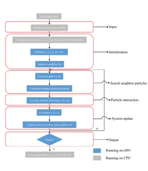
This section describes how this code is paralleled in GPU and its data structures. As is shown in Fig.2, the current GPU-accelerated model ofPCA may be divided into seven different parts which are related to input, initialization, searching neighbor particles (SNP), particle interaction (PI), system update (SU), output and writing output data. Basically, the input is designed to read information about physical parameters, such as the size of domain and initial particle size before a simulation starts. After reading input data, a kernel is launched to initialize the data, e.g. particles’ location (coordinate x and y), and velocity (v and u). Note that these data are initialized on device instead of host, which can avoid the time-consuming process of transferring data between host and device. If a code uses linked-list search algorithm to search neighbor particles, some kernels are also needed to compute the cell that a particle belongs to and the particle number in a cell (as is shown in later of this section). Neighbor searching is an essential step of a SPH algorithm. Neighbor particles must be defined and stored in a list. After building the neighbor list, all particles in the support domain of particle i can be found and the pairwise interactions among adjacent particles can be calculated. After that, all physical magnitudes describing the state of the particles should be advanced according to the interaction of particle i. When it is necessary to output the results (the calculating time or timestep is due), data are copied back to a host and written onto files in a hard drive. Initialization, searching neighbor particles, particle interaction and system update are entirely executed on the device during a simulation, which avoids communication time between host and device. The other three steps are executed on the host.
Fig. 2Flowchart of the calculation process
3.2 Nearest neighbor particle searching (NNPS) algorithm
3.2.1 All-pair search
With all-pair search algorithm, one thread corresponding to a specific particle searches all particles within the support domain to find its adjacent particles. Consider one computation domain consisting of N particles. To find particle its neighbors, a single thread need do N*(N-1)/2 calculations. If the particle number is small, little would do to the performance of GPU. However, when the number of particles increases gradually, the efficiency of GPU would reduce dramatically and the total computing time would multiply by square. For example, if it costs 1s for a thread to find neighbors in a 0.01 million particles domain, the time for a 1 million particles domain would be 10000s(nearly 3h). So the direct searching method is a time-consuming algorithm in searching neighbor particles.
3.2.2 Linked-list search
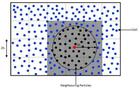
the method, all particles are firstly matched with a uniform grid with a width that equals to the maximum searching radius, normally 2 or 3 times of smoothing length. For an arbitrary particle i, all its effective neighbor particles locate in the adjacent 9 cells (consider a 2D domain) as is shown in Fig.3. So the total calculations would be about N. Surely, this method is a much more effective technic, though its data sorting strategy may be slightly complex.
Fig. 3Example of neighbor particles when using uniform grid searching method
As is shown in Fig.4, when implementing linked-list search method, each particle is given a unique index according to its location in the domain and each cell is provided with an index.
Fig. 4 Procedures to build 5 arrays.
neighbors every timestep. As a result, some arrays need to make a corresponding modification. All through the simulation, these three arrays are stored in theglobal memory of GPU, which means there is no need to make any communications between CPU and GPU. Since the costly communications can be avoided, the efficiency could be improved greatly.
During each timestep, four kernels are launched sequentially to finish the simulation. Table.1 summaries the functions of each kernel.
Table.1 Kernels and Sub-functions
Kernel Sub-functions Kernel A 1.Find neighbor particles;
2. Calculate particle interaction.
Kernel B 1.System update;
2. Advance particleIndex and particleCellNum array.
Kernel C Advance cellBegin array.
Kernel D Advance cellParticleOrder array.
Fig.5 shows the pseudo code of Kernel A. For an arbitrary particle i, its cell is found according to particleIndex array. Then its adjacent cells are found in cellNeig. After that, all particles in the cell are compared to find its neighbor particles. Lastly, the interaction between particles is calculated.
Fig.5 Pseudo code of Kernel A
When launching Kernel C, each thread corresponds to one cell. While in other kernels, each thread corresponds to one particle. So, when the particle number is big enough, it is possible to achieve a high occupancy rate in block and register, which is a useful way to hide delay and improve efficiency.
4. Model & Validation
4.1 Hardware
device, Tesla can accelerate the speed of big data analysis effectively and have been used in professional workstations and HPC clusters. Quadro GPU is specified in image processing, which is suitable for the computation and plot of complex pictures. GeForce GPU is often used in personal computers and games. The major differences between the three GPUs are the clock rate, the number of processors and the available global memory. The former two factors have a huge influence on the speed of computation, whereas the available global memory partially determines the maximum particles that can be simulated in the GPU. As for the host, these three GPUs cooperate with three different CPUs: Intel Xeon E5-2680, Intel Xeon E5-2620 and Intel Xeon E5-2650, whose clock speed are 2.4GHz, 2.1GHz and 2.6GHz respectively. The performance attributes of these particular cards are summarized in Table.2.
Table.2: GPU information and statistics
System No. 1 2 3
GPU Tesla K20c Quadro M4000 GeForce GT730
Compute Capability 3.5 5.2 3.5
Clock Rate 705.5MHz 772.5MHz 901.5MHz
Multiprocessors 13(2496 Cores) 13(1664 Cores) 2(384 Cores)
Global Memory 4096MB 8192MB 2048MB
GFLOPS(single precision) 3520 2600 690
CPU host E5-2680 E5-2620 E5-2650
CPU host clock rate 2.4GHz 2.1GHz 2.6GHz
CPU host RAM 128GB 128GB 128GB
Operating System Windows 7 64bit Windows 7 64bit Windows 7 64bit
4.2 Model
To investigate the accelerating performance of GPH for SPH, the propagation of a wave in a two-dimensional domain is simulated and the solving process is paralleled by GPU. The wave equation is presented as follow:
1
v
v
v
v
t
x
(9)
Which can be written as:
0
2 a
-( , )
exp(-(
) )
3
x t
t x
v
c
M
(10)
where t represents time (propagation starts when t= 0) and x is the geometric position. c0 is the wave propagation speed which is1 m/s. Ma is the Mach number which is 0.05
with same Y coordinate (y=0) are shown in Fig. 6.
Fig. 6 One-dimensional sound propagation model
The computation area is a 2D domain, whose x coordinate ranges from -10 to 40 and y coordinate ranges from -10 to 10.The bottom side (y=-10m) and the top side (y=10m) are set as the periodical condition which can provide a non-reflected condition for the wave’s propagation. While at the left side (x=-10m) and right side (x=40m), the particles are set free in the computation. Since the SPH computational region is far longer than the sound propagation distance, any effects caused by ignoring this boundary will not propagate to the sound propagation domain, and therefore can be neglected.
Table.3 Parameters for the SPH algorithm for sound propagation modeling.
Computational Parameters Values
dt 0.2*∆x
h 2.13*∆x
Kernel Type Gaussian
CCFL 0.20
ρ0 1.0kg/m3
During each timestep, each particle’s coordinate and velocity need to be calculated. To research the relationship between GPU’s accelerating performance and particle number, the minimum particle number in the domain is1K and the maximum is 62.5M,which can be altered by changing the initial space (∆x) between particles. In all cases, the timestep is set as dt =0.2*∆x and the smooth length takes h=2.13*∆x. The Courant-Friedriches-Lewy number is written as CCFL for short, and CCFL = u∆t / ∆x. The particle density ρ0 is 1.0kg/m3.
4.3 Validation
A code running in CPU is first proposed to verify the feasibility and accuracy of the SPH Wave propagate
method for solving wave equation problems. Note that all-pair search algorithm is used in this code. The test cases run in the No.1 system. All the results presented in this as well as the following subsection are obtained via double precision.
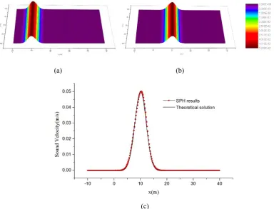
Fig.7 (a) and (b) shows the simulated results of velocity distribution at t=5s and t=10s, which clearly depicts the process of sound wave propagation. The initial space is 0.01m. The comparison between theoretical solution and simulated results along y=0 at t=5s is shown in Fig.7 (b). The theoretical solution is plotted with a solid line while the SPH results is plotted with red points. In
order to clearly identify the numerical results, the points are plotted at intervals of 12.
(a) (b)
(c)
Fig. 7 Velocity distribution. (a)t=0s, (b)t=10s, (c)the comparison along y=0 at t=10s
As shown in Fig.7, the peak of sound velocity changes along with time. It can be seen that SPH method can achieve high precision in simulating wave propagation problem. In addition, the trends of SPH results and theoretical solutions are similar.
Different computational cases are built by varying the initial space from 1m to 0.004m, and the number of particles ranges from 1K to 62.5M. The comparisons are based on the results of the100th timestep. The accuracy of SPH method can be achieved by comparing the mean square error (MSE) and the maximum error (ME) between the numerical solution and the theoretical solution. MSE and
ME are calculated as follow:
2 1
2 1
1
( ) ( )
1
( ) N
sim the i
N
the i
V i V i N
MSE
V i N
1
max sim( ) the( ) i N
ME V i V i
=
(11)
Where N is the number of particles in the computation domain, Vthe is the theoretical solution
of particle’s velocity; and Vsim is the simulation result.
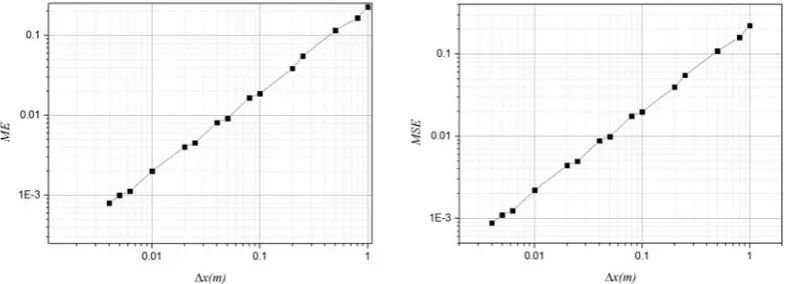
Fig. 8ME and MSE varies with the initial space in test case
Fig.8 gives the tendency of MSE and ME changing with the initial space. It can be seen from the line graph that the increasing of MSE and ME is close to linear. MSE and ME are the smallest at
the initial space ∆x = 0.004 m, which are 7.99 × 10⁻⁴ and 8.80 × 10⁻⁴ respectively. When the initial space increases, MSE and ME increase gradually too. For example, when the initial space ∆x=1m,
MSE and ME reach 0.22 and 0.21 respectively. The Convergence rate for MSE and ME is about 0.214 and 0.221 respectively. In conclusion, it is feasible to use SHP method to solve wave equation problems, and this method can obtain satisfactory accuracy.
5. Results & Discussion
5.1 All-pair search & Linked-list search
(a) (b)
Fig.9 Comparisons of runtimes. (a)runtimes of different cases, (b)speedups
As is shown in Fig.9(a), the actual runtime increases with the number of particles dramatically. For all-pair search method, when the particle numbers is 1K, the runtime is 0.15s; and when the particle numbers is 256K, the runtime is 10987s. While for linked-list search method, the runtimes are 0.07s and 25.9s respectively.
To examine the runtime difference between the algorithms, each average runtime was compared by calculating speedup for each simulation. The speedup is computed using:
lg1 lg2
=t
A/ t
A
(12)
where
t
Alg1 andt
Alg 2 are mean runtimes for algorithm 1 and algorithm 2, respectively. Fig.9(b) shows the speedup of both algorithms. There is a significant speed up gained by using algorithm 2. The speedups increase linearly with the number of particles in the computation domain. Although these two codes run in different CPUs, the speedups gained in different cases are almost the same. This comparison clearly shows the higher efficiency and advantage of using linked-list search method for nearby particles searching.
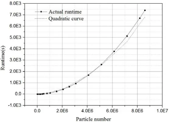
Fig. 10Runtimes for different particle numbers when using linked-list search method.
5.2 Percentage of time in different steps
In previous sector, it is clear that linked-list search method is much more efficient than all-pair search method. In the following sector, all codes use this method for searching neighbor particles, which can greatly reduce the runtime. However, SPH is still a time-consuming method. All data need to be initialized before simulating. Then there are three main steps in each timestep or a loop: searching neighbor particles (SNP), particle interaction (PI) and system update (SU). The runtimes of these steps add to the total time of a single timestep. As a consequence, it is advisable to find the most consuming step in a simulation and then paralleled the step in GPU to reduce the runtime of a simulation.
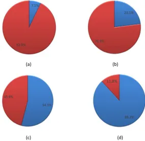
Fig.11 gives the percentage of three tasks in a loop. The runtime is the average time of 100 steps. By varying the initial space, particle numbers of the domain are 0.025M, 0.1M, 0.4M and 2.5M respectively. All the cases run on system 1.
From Fig.11, one can see that the percentage of time that three tasks use in a loop are almost the same, no matter what the particle number is. Particle interaction is the most consuming procedure, which accounts to about 53% of total runtime. Searching neighbor particle also consumes a lot of time, which takes around 43% of runtime. As for system update, it takes a very small part of total runtime, which can be omitted to some extent.
Initialization is another important procedure that may influence the total runtime in a CPU code. Since there is no need to transfer data between host and device, the time can be saved. Fig.12 shows the percentage of time that initialization and a loop cost in a simulation consisting of only one timestep. It can be seen that the percentage of initialization increases with the number of particles in a computation domain. When particle number is 0.025M, the percentage is 7.1%; while when particle number increases to 2.5M, the percentage leaps to 88.2%. Although in simulations which requires many loops the percentage declines, it is still sensible to reduce the time consumed in initialization. So the runtime of a simulation that consists of only a few steps can be reduced greatly.
In conclusion, the times devoted to initialization, searching neighbor particles and particle interaction are huge. In GPU computation, these three steps should be paralleled to reduce total runtime and to promote efficiency.
(a) (b)
(c) (d)
5.3 GPU results
In previous sections, it has been proved that it is feasible to use SPH method to solve wave equations and it can achieve a relatively high precision. Moreover, in a certain range of particle number, using linked-list search method to search neighbor particles can achieve a very high efficiency, which can save a lot of runtime compared to all-pair search method. In this section, a GPU paralleled code is proposed which uses linked-list search method for neighbor particles searching. Some of the most consuming procedures are paralleled in GPU. The detailed calculation process is shown in Chapter 3. Then, the calculation results are compared with results of the code running in CPU. The comparison shows that both results are identical.
(a) (b)
Fig. 13 Percentage of time that each task costs in cases of different particle numbers. (a)0.4M, (b)10M Table.4 The runtimes of different tasks in a simulation
Time(ms) Input Initialization SNP PI SU Output
0.025M 1008.30 1.23 1.69 8.57 0.04 0.33
0.1M 1018.80 4.66 6.70 32.18 0.15 1.06
0.4M 1019.10 18.25 26.12 118.50 0.52 3.93
2.5M 1023.20 114.20 162.20 664.60 2.99 24.16
10M 1056.30 457.70 643.30 2532.30 11.87 95.43
Fig.13 shows the percentage of time that five tasks cost in a calculation: input, initialization, SNP, PI, SU, output. Table.4 gives the detailed runtimes of all tasks. Note that all simulations involve only one timestep. As a result, it may take a relatively larger part since a simulation usually involves dozens of or even hundreds of timesteps.
So the paralleled code can greatly reduce the runtime of initialization. Data output takes a small part of the whole calculating time. When particle number is 10M, its proportion is only 2%. When particle number is relatively small, data input and initialization take a big part of the runtime. However, with the increase of particle number, there total percentage decreases dramatically. It drops from 87.45 to 31.5% when the particle number increases from 0.4M to 10M. If there are more timesteps in a simulation, its percentage will decrease more.
In a timestep, the runtimes for SNP, PI and SU increase with the number of particles linearly approximately. They are also much smaller than those of codes run on host. For instance, when particle number is 0.4M, the runtime of host is 22 times larger than that of device, which are 3186ms and 144.6ms respectively.
Table.5 Percentages of time that three tasks cost in a timestep
Percentage SNP PI SU
0.025M 16.43% 83.14% 0.43%
0.1M 17.17% 82.46% 0.37%
0.4M 18.00% 81.65% 0.36%
2.5M 19.55% 80.09% 0.36%
10M 20.18% 79.45% 0.37%
However, the particle interaction part takes a large part of the time in a timestep. As is shown in Table.5, particle interaction takes about 80% of all computing time of a timestep, though the proportion drops slightly with the increase of particle number. Searching neighbor particles only involves read data from memory without calculating. On the contrary, particle interaction needs to calculate a lot of data, such as particle distance, velocity and pressure. GPU’s calculation capacity is much inferior to CPU’s and dealing with data which are double precision consumes more time than that of single precision. As is mentioned before, all data are stored in GPU’s global memory in double precision to achieve a higher calculating precision. As a consequence, particle interaction takes much more time than searching neighbor particles and system update.
Table.6 The GPU and CPU runtimes in different cases
System No.
Particle number
CPU Runtime(min)
GPU Runtime(min)
Number of timesteps
Speedup(per timestep)
1
0.01M 26.55 1.45 100 18.3
0.25M 693.07 10.07 100 68.8
1M 2638.21 37.99 100 69.4
5M 14005.13 168.38 100 83.2
2
0.01M 35.54 2.01 100 17.7
0.25M 915.7 22.83 100 40.1
1M 3803.79 87.02 100 43.7
3
0.01M 27.25 2.68 100 10.2
0.25M 681.28 46.68 100 14.6
1M 2852.43 179.57 100 15.9
Table.6 and Figure.14 summarize the computational times and speedups in three different systems. Note that all the simulations in CPU are single-thread. As is shown in Figure.10, a significant speed up can be achieved by using GPU parallel computing. When the particle number is relatively small, the speedup increases with it dramatically. However, when the particle number is relatively large, the speedup is approximately constant. The speedups vary with different systems. As a professional scientific computing GPU, Tesla K20C can achieve good performances. For example, it can accelerate the speed of computing to 83 times when particle number is 5M. The number of particles that it can simulate is massive. For instance, it can simulate a case of 50M particles, which only takes 15s. GeForce GT730 and Quadro M4000 also show good performances, though they cannot match with Tesla K20C. In short, using GPU paralleled computing can accelerate the solving of wave equations effectively.
6. Conclusions
A parallel implementation of SPH for solving wave equations has been developed in this paper. The code is paralleled utilizing CUDA technique and is able to carry out acoustic problems with a large number of particles. The major contribution of this paper can be summarized as following:
(1) Particle-based computational acoustics is paralleled on GPU. The feasibility of this method is verified and it can achieve a desirable accuracy. All the main procedures in a simulations such as initialization, searching neighbor particles, particle interaction and system update are paralleled in GPU, which can save a lot of runtime compared with codes run in CPU.
(3) The percentages of time devoted to different procedures are analyzed to find the most time-consuming procedures. The result shows that searching neighbor particles and particle interaction take more 90% of time both in CPU and GPU.
(4) The performances of different calculating platforms which vary in CPU and GPU card are discussed. Tesla K20C is the most suitable card for paralleled calculating. It can simulate more than 50M particles in less than 15s in a timestep. When the particle number reaches 2.5M, it can get a speedup of 83.2x.
Acknowledgements
This study was partially supported by the Independent Innovation Foundation of Huazhong University of Science and Technology (No.01-18-140019) and the National Natural Science Foundation of China (No.51741910). Besides, this study was also supported by China Ship Development and Design Center (NO.9140C280105150C28001).
References:
[1] R.A. Gingold, J. Monaghan, Mon. Not. R. Astron. Soc. (1977) 375–389.
[2] Huabin Shi, Xiping Yu, Robert A. Dalrymple, Development of a two-phase SPH model for
sediment laden flows[J], Computer Physics Communications, 2017
[3] J.L. Cercos-Pita, R.A. Dalrymple, A. Herault, Diffusive terms for the conservation of mass equation in SPH[J], Applied Mathematical Modelling, Volume 40, Issue 19, 2016, Pages 8722-8736
[4] Cummins S, Rudman M. An SPH projection method[J]. J Comput Phys1999;152:584–607 . [5] JP Morris PF, Zhu Y. Modeling low Reynolds number incompressible flows using SPH[J]. J
Comput Phys 1997;136:214–26 .
[6] Monaghan J, Gingold R. Shock simulation by the particle method SPH[J]. J Comput Phys 1983;52:374–89 .
[7] Monaghan J, Gingold R. On the problem of penetration in particle methods[J]. J Comput Phys 1989;82:1–15 .
[8] Colagrossi A, Landrini M. Numerical simulation of interfacial flows by smoothed particle
hydrodynamics[J]. J Comput Phys 2003;191:448–75.
[9] Ferrari A , Dumbser M , Toro E , Armanini A . A new 3D parallel SPH scheme for free surface flows[J]. Comput Fluids 2009;38(6):1203–17.
[10] Monaghan J. Simulating free surface flows with SPH[J]. J Comput Phys 1994;110:399–406. [11] HA Posch WH , Kum O . Steady-state shear flows via non-equilibrium molecular dynamics
and smooth-particle applied mechanics[J]. Phys Rev E 1995;52:1711–19 .
Appl Mech Eng 20 0 0;184:49–65 .
[13] Valdez-Balderas D, Domínguez J M, Rogers B D, et al. Towards accelerating smoothed particle hydrodynamics simulations for free-surface flows on multi-GPU clusters[J]. Journal of Parallel and Distributed Computing, 2013, 73(11): 1483-1493.
[14] Zhang Y O, Zhang T, Ouyang H, et al. Efficient SPH simulation of time-domain acoustic wave propagation[J]. Engineering Analysis with Boundary Elements, 2016, 62: 112-122.
[15] Zhang Y O, Zhang T, Ouyang H, et al. SPH simulation of acoustic waves: effects of frequency, sound pressure, and particle spacing[J]. Mathematical Problems in Engineering, 2015, 2015. [16] Zhang Y O, Li X, Zhang T. Modeling Sound Propagation Using the Corrective Smoothed
Particle Method with an Acoustic Boundary Treatment Technique[J]. Mathematical and Computational Applications, 2017, 22(1): 26.
[17] Domínguez J M, Crespo A J C, Valdez-Balderas D, et al. New multi-GPU implementation for smoothed particle hydrodynamics on heterogeneous clusters[J]. Computer Physics Communications, 2013, 184(8): 1848-1860.
[18] Mai J. High performance computing[J]. 2011.
[19] Xia X, Liang Q. A GPU-accelerated smoothed particle hydrodynamics (SPH) model for the shallow water equations[J]. Environmental Modelling & Software, 2016, 75: 28-43.
[20] Yang Zhang, Zuocheng Xing, Cang Liu, Chuan Tang, Qinglin Wang, Locality based warp scheduling in GPGPUs, Future Generation Computer Systems, 2017, ISSN 0167-739X [21] Souley Madougou, Ana Varbanescu, Cees de Laat, Rob van Nieuwpoort, The landscape of
GPGPU performance modeling tools, Parallel Computing, Volume 56, 2016
[22] Mokos A, Rogers B D, Stansby P K, et al. Multi-phase SPH modelling of violent
hydrodynamics on GPUs[J]. Computer Physics Communications, 2015, 196: 304-316. [23] Abal-Kassim, et al, Conjugate gradient method with graphics processing unit acceleration:
CUDA vs OpenCL[J], Advances in Engineering Software, Volume 111, 2017, Pages 32-42 [24] Daniel Winkler, Michael Meister, Massoud Rezavand, Wolfgang Rauch, GPU SPH—A shared
memory caching implementation for 2D SPH using CUDA, Computer Physics Communications, Volume 213, 2017