Analysis of the Behavior of Velocity Profiles in a Standard Elbow Fitting
Víctor Places Garzón1, Bence Mátyás2,*, Luis Fernando Toapanta1**
1 Universidad Politécnica Salesiana, Quito, Ecuador
2Grupo de Investigación Mentoria y Gestión del Cambio, Universidad Politécnica Salesiana,
Cuenca, Ecuador
3Grupo de Investigación en Ciencias Ambientales, Universidad Politécnica Salesiana, Quito, Ecuador
Abstract. In this paper, we studied and analyzed the behavior of velocity profiles and the distribution of pressures in a pipe connected to an accessory. In this case, it was a 90º elbow fitting in which water flows as an incompressible flow. This study was developed numerically through the fluent program of ANSYS.
It is of practical interest in engineering because it is based on results regarding the internal structure of a model of incompressible flows. In the same way, it provides a basis for the proper design and implementation of velocity profiles within an elbow.
In the agricultural industry, suitable systems can be implemented for crop irrigation in this way with the results obtained to improve the design in the fluid distribution system.
We used a feasible κ-ε turbulence model because this model causes less turbulence than the standard κ-ε model.
A mesh independence study was developed, in which it was observed that combining different densities of meshes for the same geometry causes some variables, so a fine meshing was used to carry out the study so that the results are as close to reality as possible.
Keywords: turbulence; CFD; incompressible flow; velocity profiles
1.
INTRODUCTION
The study of hydraulic phenomena is complex and problematic. One issue is the analysis of flow velocity profiles for their various applications [1].
Fluid flow is a crucial part of performing operations in industrial plants or driving flows through geographic regions, where the effects of changing direction and velocities of fluids are of great importance [2] [3].
Simulation models of both compressible and incompressible flows are important for the analysis and design of accessories, equipment and facilities that require general fluid transport systems [4].
The optimization of hydraulic systems is based on carrying out tests and simulations for the improvement of processes [5] [6].
which a previous design must be carried out and the use of elbow fittings as a fluid diversion mechanism is completely necessary [3].
It is essential to adequately design and implement fluid driving systems in the field of agriculture, because water is a fundamental resource and extremely useful for various agricultural activities. However, optimum use is required, considering the scarcity of water in some areas. With the completion of an effective irrigation system, it is possible to use the water efficiently, ensuring quality production at the level of both small and large producers [7].
Therefore, it is important to analyze the variables that exist in the driving system, focusing on the velocity profiles generated in this type of accessory [8].
Circular section pipes are the most frequent, because their shape provides greater cross section and structural strength for the same outer perimeter than any other geometric shape [9] [10]. The many and diverse factors that influence the obtaining of a satisfactory speed in fluid systems [11] include the type of fluid, length, type of devices used, type of pipe, drops in pressure that the system can tolerate and the friction of the fluid with the duct. This was mentioned by Anaya and Segovia [12] in their investigation which analyzed the mathematical models that describe, by means of an explicit form, the friction factor for a fluid in a pipeline. They compared the numerical values of said factors with respect to the Colebrook-White equation and the Kármán number [ 12].
The flow velocity increases when the area in the flow path decreases, thus smaller diameter tubes generate high velocities and larger tubes cause low speeds [13].
In a fluid transport system it is advisable to keep the speeds low, because if speeds are too high the problem arises of friction wear on the walls, which can destroy the pipe wall and leave it exposed to corrosion [14].
In the same way, if the speed is too low, solids may plug up the pipe, reducing space within the pipe and making it difficult to operate the system [15].
Elbows are essential coupling accessories due to the changes of direction that the flow must take to give flexibility to the system [6].
When the flow leaves the elbow, the whirlpools produced by the separation create considerable pressure loss [16]. The reasons for this change of direction are based on the result you want to achieve. For example, in a heat exchanger, one needs a greater energy transfer between the fluid and the solid walls with which it is in contact; this is also true for steam generators, refrigerators, vehicle radiators and other similar systems [17] [18].
Another use of elbows within the system is the effects of mixing that are induced at the outlet of the system after passing the flow through curved passages [14].
The flow velocity in a circulating pipe can vary from one point to another of the cross section. The speed beside the pipe wall is negligible, because the fluid is in contact with the stationary pipe [19].
Studies carried out regarding conduction in curved pipes have been able to determine certain patterns that appear in the flow. Vera’s study [14] dealt in part with of the importance of numerically studying the velocity and pressure field in horizontal pipes with the use of standard elbows, where areas of slower speed inside a pipe have a combination of elbows of circular cross sections used as phase separators. This research was developed numerically using the Fluent ANSYS program.
In the same way, in his analysis, Jinés [4] studied the distribution of velocities in the three axes, turbulence, temperature, density and compressive stresses of the fluid on walls of pipes and accessories, in addition to the fluid’s energy kinetics using a program that allows one to simulate the behavior of fluids in heterogeneous conditions.
Through these studies, it has been established that when a fluid enters a curved pipe of circular, square or elliptical cross section, an imbalance occurs between the centrifugal force and the radial pressure gradient and these two factors act in opposite directions in each element of the fluid [2] [21].
This document also provides a basis for the proper design and implementation of velocity profiles within elbow fittings using software to simulate flow behavior.
2.
MATERIALS AND METHODS
2.1.
Geometric Model
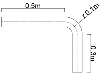
The pipe used to carry out the study is commercial steel ID no. 40, with an internal diameter of 0.0797m. It consists of 3 parts: the first is a straight 0.5m-long pipe, a 90° elbow, which has an average curvature radius of 0.10m, and finally a straight 0.3m-long pipe. This geometry is presented in figure 1. The analysis was based on velocity profiles inside the elbow with the help of a current simulator by creating a mesh and respective mathematical modeling.
2.2.
Fluid Model
Within the problem, the constant flow used was a viscous, incompressible fluid i.e. it had constant and isothermal density and the working fluid was water. Gravitational effects were considered. The specified temperature was T=20°C and the density and viscosity of water were ρ=998kg/ and μ=1.02×10 kg/(ms) respectively. These values were present in tables [20]. The flow velocity at the entrance averaged over the cross section of the pipe, V=5m/s. To determine the flow regime, the following equation (1) was used:
Re =ρVD μ
( 1)
where:
D is diameter, V is velocity, μ is dynamic viscosity and ρ is fluid density.
If the Reynolds number is relatively small, the flow is laminar; if it is large, the flow is turbulent. As one can appreciate in the definition of the Reynolds number, it is not only the flow velocity that determines the character of the flow; its kinematic viscosity and the diameter of the pipe are equally important [5].
For practical engineering purposes, the values normally taken for flows in round section pipes are the following: the flow is laminar if the Reynolds number is less than approximately 2100, it will be turbulent for numbers greater than about 4000 and between 2100 and 4000, the flow is called transition flow [14].
Upon developing equation 1, it was determined that the Reynolds number for this case was 8.6×10 , thus flow was considered to be turbulent.
2.2.
Turbulence Models
In order to obtain a better analysis, it was necessary to keep in mind the effects provoked by the turbulence. Due to this, one must use a turbulence model in the simulation process to obtain better results.
Turbulence models are generally classified according to the relevant equations, for example, Reynolds-Averaged Navier-Stokes (RANS) or Large Eddy Simulation Equations (LES). In addition, one must find a breakdown according to the number of transport equations that must be solved in order to calculate the contributions model [22].
The k-ε model is the most well-known and is used in virtually all commercial programs for fluid studies [14].
In this study, the feasible k-ε model (k-ε-r) was used.
The term feasible means that the model satisfies certain limitations in terms of normal forces, thus fulfilling the physics of the turbulent flows. To understand this, we considered and used the Boussinesq approximation and the turbulent viscosity definition to obtain the following expression for Reynolds normal force in an incompressible flow:
⃐ =2
3 − 2
⃐ ( 2)
⃐ =2
3 − 2
⃐ ( 2)
The feasible k-ε model differs from traditional k-ε models, due to the following- it has a new equation for turbulent viscosity, involving the variable Cμ, originally proposed by Reynolds, and a new equation for the dissipation of turbulent kinetic energy, based on the equation of the mean root of the fluctuation of the vorticity.
The turbulent kinematic viscosity is obtained:
≡
( 3)
⃐ > 1
3 ≈ 3.7 ( 4)
Therefore, the equations for the feasible k-ε are the following: equation 5 for (k) and equation 6 for (ε).
⃐
+ ¯
= + + + + +
− −
⃐
+ ¯
= + + + +
−
+ √ +
( 6)
where:
= 0.43
+ 5 ( 7)
=
( 8)
≡ 2
( 9)
The difference between the k-ε model and the feasible k-ε model is that Cμ is not constant; its formula is now:
= 1
+ ∗ (10)
where:
∗≡ 2 + ~ ~
(11)
~
= − 2
(12)
In these proposed equations, represents the generation of turbulent kinetic energy due to low velocity gradients. describes the generation of turbulent kinetic energy produced by flotation. represents the generation of energy due to fluctuating compression in turbulent compressible flows.
In the same way, Ω = Ω~ − Ω~ is the rotation tensor seen from the reference point of the angular velocity ( ).
∅ =1
3 √6 (13)
= ~
(14)
~ =
(15)
~ =1
2 ⃐
+ ⃐
(16)
, , are constants. y are Prandtl numbers for k and ε respectively. The coefficients that one obtains are the following:
= 1.44, = 1.9, = tan
¯
, = 1.0, = 1.2
4.
RESULTS AND DISCUSSION
4.1.
Multiphase bypass meshing
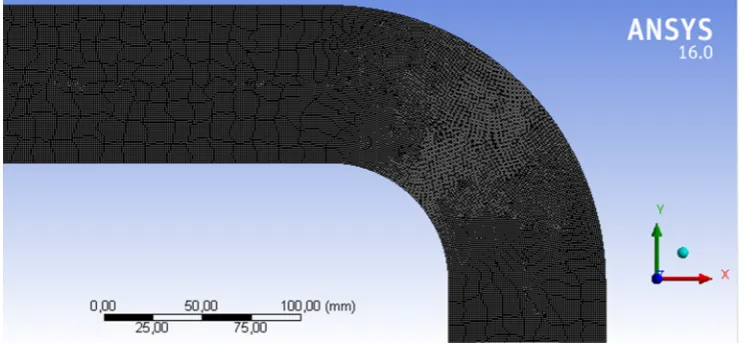
Meshing is one of the most important parts for the purpose of simulation as results will also depend on its quality. Once the 2D drawing of the elbow is completed, one proceeds to the meshing stage. The smaller the cells, the more the simulation will reflect reality.
Through the multiphase flow evaluated with Fluent of ANSYS, in this study, the effect of velocity, pressure and turbulence in commercial steel tubes was analyzed using the κ-ε model with a velocity of 5m/s. All this will be detailed later with various graphs in the results section. The fluid that we worked with was liquid water at a temperature of 20°C and the simulations were carried out with Fluent in 2D due to the high computational resource that simulations in 3D provoke. Figure 2 shows the mesh of the elbow.
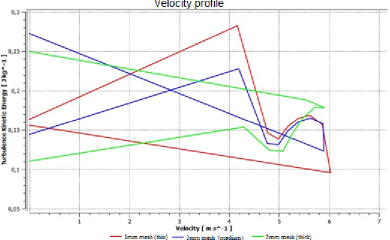
An important aspect in CFD is the independence of the mesh, which is based on the fluid velocity (see figure 3). There are three different velocity profiles depending on the mesh size, which can be thin, medium and thick, corresponding to 1, 3 and 5mm respectively, where fine meshing improves the flow velocity profile. Due to this, when working with fine mesh, calculations are most approximate to reality. The analysis for the mesh independence was carried out at the accessory’s outlet at the end of the curve.
Figure 3. Independence of the mesh, based on velocity.
Source: Authors
From this point on, the results obtained in the elbow were with the fine mesh, because of the characteristics and advantages that it provides in comparison to the medium and thick mesh. The convergence of the residuals is the first step in validating the solution since it must converge in order for one to know that the iterations made are correct and the answers obtained will be reliable.
Table 1. Characteristics of the different meshes
Source: Author
Mesh Type No. of Iterations No. of Nodes
1mm mesh (thin) 982 77669
3mm mesh (medium) 174 9009
Table 2 details some characteristics obtained with the variation of the mesh thickness. It was possible to highlight that the difference between the number of nodes of each mesh varies drastically, so the results would also vary.
4.2.
Numerical Simulation of the Fluid
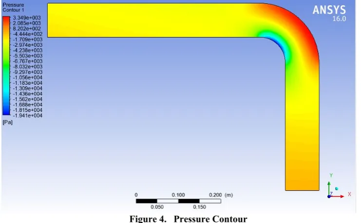
The graphs of turbulence, velocity, static pressure and others, which are detailed below and each represent the behavior that registered the fluid flow inside the accessory with the fine mesh and the variables at the entrance of the elbow, such as the velocity, temperature and Pressure.
Figure 4. Pressure Contour Source: Authors
Figure 5. Turbulence Contour Source: Authors
Figure 5 shows a distribution of turbulence at the end of the pipe; at the outlet, the turbulent effects descend the section. There is greater turbulence at the curvature outlet.
When the flow of a fluid enters an accessory, in this case a 90° elbow, the velocity profile is affected, meaning that in certain parts of the accessory the flow is accelerated and in other parts decelerated.
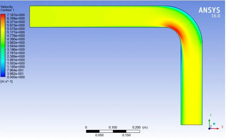
Figure 6. Velocity Contour Source: Authors
vortex viscosity and velocities then diffuse until the original distribution is recovered, although the effect of the elbow can still be observed at a great distance downstream. One can appreciate that lower velocities occur in the area of greater radius within the accessory, because in this part there is greater friction with the wall which causes it to slow down.
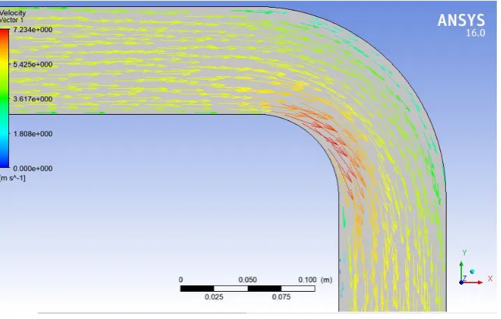
Figure 7. Velocity Vector Source: Authors
Figure 7 presents a distribution of the velocity vectors in the internal structure of the pipe and the accessory. An approximation is made, where the direction in the flow was noticed, as well as which vectors show more deviation in the accessory.
5.
CONCLUSIONS AND RECOMMENDATIONS
It is important to analyze the velocity profiles and directions that the vectors take because this allows one to evaluate some problems that may occur due to the fluid that circulates inside the elbow.
The implementation of elbows is necessary in adequate systems for crop irrigation. Both small and large producers can implement systems with the results obtained to improve the design in the fluid distribution system in order to prevent damages to the system which may occur and in the same way prevent crop production from being affected.
The profile of static pressure is important, because it shows the distribution of the flow that takes place in the accessory. Forces are applied at their maximum values in this region,
demonstrating reliability in the simulation.
Small meshes are recommended so that there is a greater number of nodes and the results obtained are completely reliable.
6.
REFERENCES:
[1] A. B. R. y. M. Pérez, Fundamentos y aplicaciones de la Mecánica de Fluidos, Sevilla:
McGraw-Hill , 2005.
[2] S. Felder y H. Chanson, «Turbulent air-water flows in hydarulic structures: Dynamic similarity and scale,» de Environmental Fluid Mechanics, 2009, p. 18.
[3] C. Ed, Flujo de fluidos en válvulas, accesorios y tuberías., Madrid: McGraw Hill, 1997.
[4] J. Jines, «Simulación de Flujo Incompresible y de una Fase en Accesorio de Tuberias
mediante dinámica de fluido computacional,» Revista Tecnológica ESPOL, vol. 30, nº N. 2, 56-74, p. 19, 2017.
[5] b. Nicolás D. Badano y Á. N. Menéndez, «Evaluación Numérica de los Efectos de Escala
de Reynolds en un Codo a 90º,» de Laboratorio de Modelacián Matemática, Facultad de
Ingeniería, Universidad de Buenos Aires, Buenos Aires, 2016, p. 16.
[6] J. C. Garzón Cruz, «Universidad EIA,» 20 enero 2014. [En línea]. Available:
http://fluidos.eia.edu.co/hidraulica/articuloses/flujoentuberias/reducci%C3%B3n/reducci%C 3%B3n.htm.
[8] D. S. Miller, Internal Flow Systems, Cranfield: BHRA, 1990.
[9] V. L. Streeter, Mecánica de fluidos, México: McGraw-Hill, 1970.
[10] R. V. Giles, Mecánica de Fluidos e Hidraulica, México D.F: McGraw-hill, 1994.
[11] A. Crespo, Mecánica de fluidos, Madrid: Paraninfo, 2006.
[12] A. Anaya-Durand, I. Cauich-Segovia, I. Funabazama-Bárcenas y O. & Gracia-Medrano- Bravo, «Evaluación de ecuaciones de factor de fricción explícito,»
[13] I. H. SHAMES, La mecánica de los fluidos, México D.F: McGraw Hill , 1995.
[14] V. R. V. ARENAS, «ESTUDIO NUMERICO DEL CAMPO DE VELOCIDAD Y DEPRESIONES EN TUBERÍAS HORIZONTALES CON COMBINACIÓN DE CODOS
DE 90°,» de Laboratorio de Ingeniería Térmica e Hidráulica Aplicada, México D.F., 2006, p. 106.
[15] C. J. RENEDO, «Universidad Cantabria,» 07 2015. [En línea]. Available:
http://personales.unican.es/renedoc/Trasparencias%20WEB/Trasp%20Termo%20y % 20MF/00%20GRADOS/MF%20T04.pdf. [Último acceso: 09 10 2017].
[16] (Unet), Universidad de Venezuela, «Flujos en tuberias,Flujos Internos,» AISC, Madrid, 2016.
[17] R. A. P. y. A. E. Larreteguy, Ajuste de perfiles de velocidad para flujo en tuberías,
Buenos Aires, 2002, p. 20.
[18] J. Franzini y E. Finnemore, Mecánica de fluidos,con aplicaciones en ingeniería, España: Mc Graw-Hill, Inc, 1999.
[19] unet.edu, «unet.edu,» 10 2010. [En línea]. Available:
http://www.unet.edu.ve/~fenomeno/F_DE_T-153.htm. [Último acceso: 25 10 2017].
[20] R. L. Mott, Mecánica fe fluidos, México: Pearson educación, 2006.
[21] M. Montilva, «Flujo Laminar en la Región de entrada de un tubo recto precedido por una tuberia curva,» Venezuela, 2009.
[22] G. F. Homicz, «Computational fluid dynamic simulations of pipe elbow flow,» Sandia National Laboratories , Albuquerque, 2004.
[23] B. R. Munson y D. F. Young, Fundamentos de Mecánica de Fluidos, México D.F: Limusa Wiley, 1999.