Deviation pattern approach for optimizing perturbative terms of QCD renormalization group invariant observables

Deviation pattern approach for optimizing perturbative terms of

QCD renormalization group invariant observables

M.R.Khellat1_{andA.Mirjalili}1

1_{Physics Department, Yazd University, P.O.Box, 89195-741, Yazd, Iran}

Abstract.We first consider the idea of renormalization group-induced estimates, in the context of optimization procedures, for the Brodsky-Lepage-Mackenzie approach to gen-erate higher-order contributions to QCD perturbative series. Secondly, we develop the de-viation pattern approach (DPA) in which through a series of comparisons between lower-order RG-induced estimates and the corresponding analytical calculations, one could modify higher-order RG-induced estimates. Finally, using the normal estimation pro-cedure and DPA, we get estimates ofα4

scorrections for the Bjorken sum rule of polarized deep-inelastic scattering and for the non-singlet contribution to the Adler function.

1 Introduction

One of the main objectives of studying different ways of optimizing perturbative expansions for phys-ical quantities is to disclose critphys-ical information about the sources of ambiguities that arise at diff er-ent orders in perturbation theory studies. The limits and validity of these perturbative descriptions is another theoretical challenge which should be addressed particularly in a complete optimization prescription. Consequently, unambiguous determination of the factorization scale would be crucial. Light-front holographic formalism is an instance of a complete optimization prescription which de-fines an effective coupling for hadron dynamics at all momenta and takes advantage of the principle of maximum conformality (PMC) [1–3] to fix the renormalization scale ambiguity. A review of this program alongside its current status and existing debates, such as the alternatives to PMC, can be found in [4].

Moreover, important investigations have been going on for several years by the authors of [5–9] to understand the consequences of considering a conformal symmetry (CS) limit in QCD. The objective of these investigations involves: to find at first a plausible generalization of the Brodsky-Lepage-Mackenzie (BLM) approach which is capable of resumming charge renormalization contributions in QCD perturbative series at different orders, and secondly clarify whether PMC, in the CS limit, gen-erates series with scheme-independent coefficients. As a result of these investigations, an extension of the BLM approach, called sequential-BLM (seBLM), has been developed and evaluated in [5, 7]. The procedure of seBLM is formulated based on the proposed{β}-expansion for QCD observables and resums theβ-dependent terms into a single renormalization scale through the renormalization-group equation (RGE) by rearranging these terms in several stages. It should be mentioned that the original

version of PMC assumes aβ-representation for the coefficients of QCD perturbative series which is different from the{β}-expansion of seBLM; however, PMC-II employs the same combination of β coefficients as seBLM and performs a resummation of theβ-pattern into different scales at different orders [10, 11].

In addition, to resolve the issue of scheme-invariance, PMC-II suggests an analogy between the general structure of a QCD perturbative series and the induced terms in the structure of the series when the series is expressed in aRδscheme [10], as a subclass of the minimal subtraction schemes. The characteristic of this class of MS-like schemes is that they are related to each other through scale transformations. In fact, scheme-dependence of the BLM approach, as the predecessor of PMC, has been previously discussed in several cases [12–14]. Probably, PMC-II follows the strategy of identifying a class of plausible schemes, which translate their renormalization scales into each other, as a remedy to demonstrate a relation between scheme and scale ambiguities. However, this point should be considered cautiously even within theRδschemes.

The next important theoretical criteria regarding any formulation of an optimization prescrip-tion is whether that formulaprescrip-tion respects the general structure of perturbative expansions and the renormalization-group or not. A carefully established estimation procedure is potentially capable of revealing such characteristics of an optimization formulation. Motivated by the renormalization group equation, the idea of RG-inspired estimates was developed in [15] to generate estimates for scheme-independent optimization prescriptions in QCD. We would devise a similar plan for the BLM scale-fixing procedure in which one would adopt a series of estimates for a renormalization group invariant observable at different orders up toO(αn

s). After this stage, we would modify the∼ αis,2 ≤ i ≤ n estimate to produce an estimate at∼αn+1

s . To generate an (i+1)-th order estimate, we start from the i-th order BLM scale-fixed series and evolve the series using the (i+1)-th order RGE.

2 The procedure of estimation

Consider a RG invariant perturbative expansion in an MS-like scheme asR(Q2_{)= r}

0+r1as(Q2)+

_∞

i=2riasi(Q2) for which the normalizationas = αs/π has been chosen. At any order, this series is supposed to represent a measurable quantity within that order of perturbative approximation. On the other hand, due to the renormalization procedure, the truncated series has become a function of the renormalized parameters. To resolve the issue, one could take advantage of the BLM proposal to assign a single renormalization scale or multiple scales at different orders for the series. Here, we follow the single scale extension of BLM proposed in [16] and extend the corresponding definition of the BLM scale to any order through the following recursive relation [17]

(k) _≡lnμ2

BLM/μ20

=(k−1)₊

k−2

i=0

ckiakp−2(μBLM). (1)

In (1) the NLO and N2_{LO BLM scales and coefficients, corresponding tok =2 andk =3, can be}

adopted from [17]. Taking the N(k−1)_{LO BLM scale-fixed series}

R(_BLMk) =r0+r1ap(μBLM)+r¯2a2p(μBLM)+. . .+r¯kakp(μBLM),

one could evolve the series using the RG equation at order (k+1)

μ2 da

dμ2 =−

k−1

i=0

βia(μ)i+2,

a(μ0)=exp

−(k)_β(a)∂

a

where the operator representation of [5] has been adopted to formulate the evolution of the renormal-ized coupling through the renormalization scales.

Here, we would formulate our procedures based on thenf expansionri =

i−1

k=0riknkf for the co-efficients of the RG-invariant expansion. However, we should note that any implementation of BLM should obey its core principle to resum vacuum polarization contributions, which are accumulated in the{β}-coefficients of the renormalization scheme. The trick to take care of vacuum polarization insertions by resumming flavor-dependent terms would not work at N4_{LO and beyond wheren}1

f

con-tributions start to appear which are not related to charge renormalization. As a result, our proposed formulation is restricted to be valid up to N4_LO.

N2_{LO and N}3_{LO estimates equivalent tok =3 andk=4 can be found in (1,8) from [17]. For}

instance, the analyticalSU(Nc) expression for the N2LO estimate would be

r₃(est) =−121 16 C2 A T2 F r2 21

r1 −

17 8

C2

A TF

r21 −

11 2

CA TF

r20r21

r1

+

2r20r21 r1

+5 4r21CA+

3 4r21CF

nf + r2

21

r1

n2_f . (3)

Here [Ta_,Ta_]

i j =CFδi jandfacdfbcd =CAδabare quadratic Casimir operators of the fundamental and adjoint representations of the color groupSU(Nc) and tr(TaTb)=TFδabis the trace normalization of the fundamental representation;{CF = N

2

c−1

2Nc ,CA =Nc,TF =1/2}. As it is also explained in the next section,∼a3 _and∼a4_{estimates in [17] are generated by the inverse of (2) as an operator equation}

atO(α3

s) andO(α4s)-levels incorporating(1)and(2), respectively. The third-order estimation is given by (3) in which the presence of−(1) _{= −3r}

21/TFr1 is evident. It should also be noted that, in this

framework, transition fromnf expansion to seBLM{β}-pattern would not be possible.

The most important characteristic of these N2_{LO and N}3_{LO estimates is that they vanish}

com-pletely at the perturbative quenched QED (pqQED) limit{CF =1,CA =0,TF =1,nf =0}. We refer the reader to a detailed study of the pqQED model, the specifications of the conformally invariant limit of the model. Its connection with the consideration of massless perturbation theory results, obtained in pqQED can be found in [18].

2.1 Deviation pattern approach

For generating the exact NkLO results from a Nk−1_{LO BLM scale-fixed series, we need}(k) _{and ¯r}

k; however, we just have access to(k−1)_{and the estimates are generated on the basis of ¯r}

k=0. In other words, estimates are naturally deviated from the exact results. On the other hand, these deviations occur at all orders and, for purely numerical purposes, we can take advantage of our knowledge of the deviation of lower-order estimates from the exact results. A possible algorithm which could directly include deviations in the estimation procedure by performing numerical comparisons and modifications would be,

1. k=2 estimation and modification:

(a) generate the N2_{LO estimate via (3)}

(b) make the comparisonr(₃est) =r(₃exact)which is equivalent to the following three equations

r(₃₀exact) = r(₃₀est) = −121 16 C2 A T2 F r2 21 r1 − 17 8 C2 A TF

r21 −

11 2

CA TF

r20r21

r1

,

r₃₁(exact) = r₃₁(est) = 2r20r21 r1 +

5 4r21CA+

3

4r21CF, r

(exact)

32 = r

(est)

32 =

r2 21

r1

(c) solve the three equations for{r1,r20,r21}and substitute the solutions in the expression for

r(₄est); the modification is like changing the weights of the constituents ofr(₄est).

2. k>2 estimations and modifications (suppose we have access to exact results up to NkLO ):

(a) generate N2_{LO to N}k_{LO estimates, i.e.k−1 estimates.}

(b) make the comparisons{r(_jest)=rj,3≤ j≤k+1}which are equivalent to 3+4+. . .+k= (1/2)(k−1)(k+4) equations{r(mnest)=rmn(exact)}for 3≤m≤k+1 and 0≤n<m.

(c) perform a selection of equations because the number of free parameters controlling the es-timates is (k/2)(k+1); therefore, (k−2) comparisons should be left out (for an explanation of the point in 4th order estimations, see section 2.2 in [17]).

(d) adapt (k/2)(k+1) parameters obtained from the previous step to modifyr(_kest₊₂).

3 Adler function and Bjorken sum rule

The primary building block of the Adler function andR-ratio is the vacuum polarization function Π(Q2_{) which is a scale-dependent object in QFT and in the MS-scheme is a function of the}

renormal-ization scaleμand the running couplingas

(qμqν−q2gμν)Π(Q2)=i

d4xeiq.x0|T[jμ(x)jν(0)]|0.

HereQ2 _{= −q}2 _{and the time-dependent correlator is responsible for the production of the vacuum}

polarization. The Adler function andR-ratio are related to the vacuum polarization function and the hadronic EM vacuum polarization function as follow [19, 20]

D(Q2_)=−12π2_Q2 d

dQ2Π(Q 2_),

˜

R(s)=6πΠE M(−s−i))−ΠE M(−s+i) . (4)

These two functions are related to each other through the well-known integral transformations

D(Q2₎₌

_∞

0

Q2_{R(s) ds˜}

(s+Q2₎2, R(s)˜ =

i 2π

s+i

s−i dz

z Dpt(−z). (5)

The corresponding perturbative expansionsDpt(Q2) = nd pt

nαns(Q2) and ˜R(s) =

nr˜nαns(s) would also become connected by introducing appropriate analytical continuation procedures [21].

The Bjorken polarized sum rule is an integration over the difference between proton and neutron polarized structure functions[22]

Γp−n

1 =

1

0

dx g₁p(x,Q2)−gn₁(x,Q2)

= gA 6 C

B jp_(Q2₎₊ ∞

j=2

μp−n

2j (Q2) Q2j−2 .

Table 1.CnsB jpandDns∼a4estimates

CB jp n0

f n1f n2f n3f D

NS _n0

f n1f n2f n3f

cest

4 -265.4 95.26 -5.94 0.08 d

est

4 362.1 -99.08 5.04 -0.05

cest1

4 -261.3 67.71 -3.62 0.04 d

est1

4 317.2 -93.26 4.76 -0.03

cexact

4 -479.4 123.4 -7.69 0.10 d

exact

4 407.4 -103.3 5.63 -0.03

in the MS-scheme,

Dns(as)=1+d1as+d2a2s+d3a3s+d4a4s+O(a5s), (6)

CnsB jp(as)=1+c1as+c2a2s+c3a3s+c4a4s+O(a5s). (7)

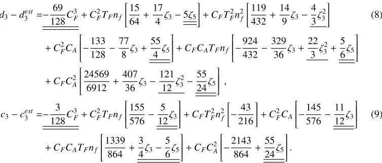
It would be convenient to compare the exact results for the color structures at N2_{LO approximation}

with the color structures of the respective estimated contributions to these functions, i.e. d3 andc3

withdest

3 andcest3 . We could write the corresponding differences as follows:

d3−dest3 =−

69 128C

3

F+C

2

FTFnf

15 64+

17 4 ζ3−5ζ5

+CFT2Fn2f

119 432 +

14 9 ζ3−

4 3ζ 2 3 (8)

+C2

FCA

⎡ ⎢⎢⎢⎢⎢

⎣−133₁₂₈ −77₈ ζ3+

55 4 ζ5

⎤ ⎥⎥⎥⎥⎥

⎦+CFCATFnf

⎡ ⎢⎢⎢⎢⎢

⎣−924₄₃₂−329₃₆ζ3+

22 3 ζ

2

3 +

5 6ζ5

⎤ ⎥⎥⎥⎥⎥ ⎦

+CFC2A

⎡ ⎢⎢⎢⎢⎢

⎣24569₆₉₁₂ +407₃₆ζ3−

121 12 ζ

2

3−

55 24ζ5

⎤ ⎥⎥⎥⎥⎥ ⎦ ,

c3−cest3 =−

3 128C

3

F+C2FTFnf

⎡ ⎢⎢⎢⎢⎢

⎣155₅₇₆ −₁₂5 ζ3

⎤ ⎥⎥⎥⎥⎥

⎦+CFTF2n2f

−43 216

+C2_FCA

⎡ ⎢⎢⎢⎢⎢

⎣−145₅₇₆−11₁₂ζ3

⎤ ⎥⎥⎥⎥⎥

⎦ (9)

+CFCATFnf

⎡ ⎢⎢⎢⎢⎢

⎣1339₈₆₄ +3₄ζ3−

5 6ζ5

⎤ ⎥⎥⎥⎥⎥

⎦+CFC2A

⎡ ⎢⎢⎢⎢⎢

⎣−2143₈₆₄ +55₂₄ζ5

⎤ ⎥⎥⎥⎥⎥ ⎦.

The terms which are double-underlined do exclusively belong to the exact analytical resultsd3andc3

while the terms proportional toζ2

3 in (8) belong todest3 . Transcendental Riemann functions related to

the Bjorken sum rule of the polarized lepton-hadron DISCnsB jpstart to appear at∼a3 while forDns they exist at∼a2_{; this is the reason why there are noζ}

3andζ5contributions incest3 .

Having an input on the difference between N2_{LO estimates ofD}ns_andCB jp

ns and the corresponding exact results, it would be possible to follow the estimation procedure of Sec. 2 and the deviation pattern approach in Sec. 2.1 to produce N3_{LO estimates for these functions in table 1. The est}

superscript refers to the method of Sec. 2 andest1 superscript to the DPA estimates. As listed in the table, one can also find the exact numerical results for bothDns(Q2_{) [20] andC}B jp

ns (Q2) [23] at the fourth-order of perturbative approximation.

References

[1] S. J. Brodsky and L. Di Giustino, Phys. Rev. D86, 085026 (2012)

[2] S. J. Brodsky and X. G. Wu, Phys. Rev. D85, 034038 (2012). Erratum: [Phys. Rev. D86, 079903 (2012)]

[3] S. J. Brodsky, M. Mojaza and X. G. Wu, Phys. Rev. D89, 014027 (2014) [4] S. J. Brodsky, J. Few-Body Syst.57, 703 (2016)

[5] S. V. Mikhailov, JHEP0706, 009 (2007)

[6] A. L. Kataev and S. V. Mikhailov, Theor. Math. Phys.170, 139 (2012) [7] A. L. Kataev and S V. Mikhailov, Phys. Rev. D91, 014007 (2015) [8] G. Cvetic and A. L. Kataev, Phys. Rev. D94, 014006 (2016) [9] A. L. Kataev and S. V. Mikhailov, JHEP1611, 079 (2016)

[10] M. Mojaza, S. J. Brodsky, and Xing-Gang Wu, Phys. Rev. Lett.110, 192001 (2013) [11] Hong-Hao Ma et al., Phys. Rev. D91, 094028 (2015)

[12] W. Celmaster and P. M. Stevenson, Phys. Lett. B125, 493 (1983) [13] J. Chyla, Phys. Lett. B356, 341 (1995)

[14] S. J. Brodsky, V. S. Fadin, V. T. Kim, L. N. Lipatov, and G. B. Pivovarov, JETP Lett.70, 155 (1999)

[15] A. L. Kataev and V. V. Starshenko, Mod. Phys. Lett. A10, 235 (1995) [16] G. Grunberg and A. L. Kataev, Phys. Lett. B279, 352 (1992)

[17] A. Mirjalili and M.R. Khellat, Int. J. Mod. Phys. A29, 1450178 (2014) [18] A. L. Kataev, JHEP1402, 092 (2014)

[19] S. L. Adler, Phys. Rev. D10, 3714 (1974)