Article
1
Map Archive Mining: Visual-analytical Approaches
2
to Explore Large Historical Map Collections
3
Johannes H. Uhl 1,*, Stefan Leyk 1, Yao-Yi Chiang 2, Weiwei Duan 2 and Craig A. Knoblock 2
4
1 Department of Geography, University of Colorado Boulder, Boulder, Colorado, USA;
5
{johannes.uhl;stefan.leyk}@colorado.edu
6
2 Spatial Sciences Institute, University of Southern California, Los Angeles, California, USA;
7
{yaoyic;weiweidu;knoblock}@usc.edu
8
* Correspondence: [email protected]; Tel.: +01-303-492-2631
9
Abstract: Historical maps constitute unique sources of retrospective geographic information.
10
Recently, several map archives containing map series covering large spatial and temporal extents
11
have been systematically scanned and made available to the public. The geographic information
12
contained in such data archives allows extending geospatial analysis retrospectively beyond the era
13
of digital cartography. However, given the large data volumes of such archives and the low
14
graphical quality of older map sheets, the processes to extract geographic information need to be
15
automated to the highest degree possible. In order to understand the salient characteristics, data
16
quality variation, and potential challenges in large-scale information extraction tasks, preparatory
17
analytical steps are required to efficiently assess spatio-temporal coverage, approximate map
18
content, and spatial accuracy of such georeferenced map archives across different cartographic
19
scales. Such preparatory steps are often neglected or ignored in the map processing literature but
20
represent highly critical phases that lay the foundation for any subsequent computational analysis
21
and recognition. In this contribution we demonstrate how such preparatory analyses can be
22
conducted using classical analytical and cartographic techniques as well as visual-analytical data
23
mining tools originating from machine learning and data science, exemplified for the United States
24
Geological Survey topographic map and Sanborn fire insurance map archives.
25
Keywords: map processing; retrospective landscape analysis; visual data mining, image retrieval,
26
low-level image descriptors, color moments, t-distributed stochastic neighborhood embedding,
27
USGS topographic maps, Sanborn fire insurance maps
28
29
1. Introduction
30
Historical maps contain valuable information about the Earth’s surface in the past. This
31
information can provide a detailed understanding of the evolution of the landscape as well as the
32
interactions between and the drivers of geographic phenomena, such as human-made structures (e.g.,
33
transportation networks, settlements), vegetated land cover (e.g., forests, grasslands) or
34
hydrographic features (e.g., stream networks, water bodies). However, this spatial information is
35
typically locked in scanned map images and needs to be extracted to get access to the geographic
36
features of interest in machine readable data formats that can be imported into geospatial analysis
37
environments.
38
Map processing, or information extraction from digital map documents, is a branch of document
39
analysis that focuses on the development of methods for the extraction and recognition of information
40
in scanned cartographic documents. Map processing is an interdisciplinary field that combines
41
elements of computer vision, pattern recognition, geomatics, cartography, and machine learning. The
42
main goal of map processing is to “unlock“ relevant information from scanned map documents to
43
provide this information in digital, machine-readable geospatial data formats as a means to preserve
44
the information digitally and facilitate the use of these data for analytical purposes [1].
45
2 of 17
Remotely sensed earth observation data from space and airborne sensors has been
46
systematically acquired since the early 1970s and provides abundant information for the monitoring
47
and assessment of geographic processes and how they interact over time. However, for the time
48
periods prior to operational remote sensing technology, there is little (digital) information that can
49
be used to document these processes. Thus, map processing often focuses on the development of
50
information extraction methods from map documents or engineering drawings created prior to the
51
era of remote sensing and digital cartography, thus expanding the temporal extent for carrying out
52
geographic analyses and landscape assessments to more than 100 years in many countries.
53
Information extraction from map documents includes the steps of recognition (i.e., identifying
54
objects in a scanned map such as groups of contiguous pixels with homogeneous semantic meaning),
55
and extraction i.e., transferring these objects into a machine-readable format (e.g., through
56
vectorization). Extraction processes typically involve image segmentation techniques based on
57
histogram analysis, color-space clustering, region growing or edge detection. Recognition in map
58
processing is typically conducted using template matching techniques involving shape descriptors,
59
cross-correlation measures or based on feature descriptors. Exemplary applications of map
60
processing techniques include the extraction of buildings [2-4], road networks [5], contour lines [6],
61
composite forest symbols [7] or the recognition of text from map documents [8,9]. Most approaches
62
rely on handcrafted or manually collected templates of the cartographic symbol of interest and
63
involve a significant level of user interaction, which impedes the application of such methods for
64
large-scale information extraction tasks where high degrees of automation are necessary to process
65
documents with high levels of variation in data quality.
66
The availability of abundant contemporary geospatial data for many regions of the world offers
67
new opportunities to employ contemporary geospatial data as ancillary information to facilitate the
68
extraction and analysis of geographic content from historical map documents. Such approaches
69
include the use of contemporary spatial data for georeferencing historical maps [10], assessing the
70
presence of objects in historical maps across time at locations dictated by contemporary geospatial
71
vector data [11], or the automated collection of template graphics for cartographic symbols of interest
72
based on locations derived from modern geospatial data sources [12].
73
Most existing approaches for content extraction from historical maps still require a certain
74
degree of user interaction to ensure acceptable extraction performance for individual map sheets, e.g.
75
[13]. To overcome this persistent limitation, [14] and [15] propose the use of active learning and
76
similar interactive concepts for more efficient recognition of cartographic symbols in historical maps,
77
whereas [16] examine the usefulness of crowd-sourcing for the same purpose.
78
Moreover, the recent developments in deep machine learning in computer vision and image
79
recognition have catalyzed the use of such techniques for geospatial information extraction from
80
earth observation data [17-26]. This methodological development naturally projects into the idea of
81
applying state-of-the-art machine learning techniques for information extraction from scanned
82
cartographic documents, despite their fundamentally different nature compared to remotely sensed
83
data. Key in both cases is the need for abundant and representative training data which requires
84
automated sampling techniques. First attempts in this direction have used ancillary geospatial data
85
for the collection of large amounts of training data in historical maps [27-30].
86
Besides this, several efforts have recently been conducted in different countries to systematically
87
scan, georeference, and publish whole series of topographic and other map documents. These
88
developments include efforts at the United States Geological Survey (USGS), that scanned and
89
georeferenced approx. 200,000 topographic maps published between 1884 and 2006 at different
90
cartographic scales between 1:24,000 and 1:250,000 [31] and the Sanborn fire insurance map collection
91
maintained by the U.S. Library of Congress, that contains more than 500,000 sheets of large-scale
92
maps of approximately 12,000 cities and towns in the U.S., Canada, Mexico, and Cuba, out of which
93
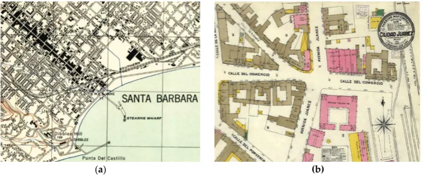
approximately 6,000 map sheets have been published as scanned map documents [32-34]. Figure 1
94
shows an example of a USGS topographic map sheet and a Sanborn map, respectively. Furthermore,
95
map sheets and town plans for the United Kingdom dating back to the 1840s and provides many of
97
them as seamless georeferenced raster layers [35,36].
98
99
(a) (b)
Figure 1. Examples of historical map documents: (a) USGS topographic map 1:31,680 from Santa
100
Barbara (California, 1944) and (b) Sanborn fire insurance map from city center of Ciudad Juárez
101
(Mexico, 1905).
102
These developments, alongside with advances in the processing, storage and distribution of
103
large data volumes, offer great potential for automated, large-scale information extraction from
104
historical cartographic document collections in order to preserve the contained geographic
105
information and make it accessible for geospatial analysis. Because of the large amount of data
106
contained in these map archives, high degrees of extraction automation are necessary. This
107
constitutes a challenging task given the high variability in the content and quality of maps within an
108
archive. Possible reasons for such variability are different conditions of the archived analogue map
109
documents, differences in the scan quality, as well as changes in cartographic design best practices
110
that may have resulted in different symbologies over multiple map editions (Figure 2).
111
112
113
Figure 2. Example of the multi-temporal, multi-scale USGS topographic map archive, showing
114
available map sheets covering Boulder, Colorado (USA) from 1904 to 2013 at various map scales.
115
The challenges described above summarize some of the central tasks in map archive processing
116
which include dealing with the sheer data volume, the differences in cartographic scales and designs,
117
changes in content and cartographic representations and their degree of similarity in individual
118
maps, the spatial and temporal coverage of the map sheets, and the spatial accuracy of the
119
georeferenced map which dictates the degree of spatial agreement to contemporary geospatial
120
ancillary data. While the previously described approaches represent promising directions towards
121
higher levels of automation, they imply that the graphical characteristics of the map content to be
122
4 of 17
across the processed map documents. Typically, many of these aspects are a priori unknown, since
124
such large amounts of data cannot be analyzed manually. However, these are relevant pieces of
125
information to better understand the data sources in order to design effective information extraction
126
methods.
127
The remote sensing community faces similar challenges. The steadily increasing amount of
128
remotely sensed earth observation data requires effective mining techniques to explore the content
129
of large remote sensing data archives. Therefore, visual data mining techniques have successfully
130
been used to comprehensively visualize the content of such archives. Such image information mining
131
(IIM) systems allow to discover and retrieve using available metadata, and based on the similarity of
132
the content of the individual datasets, or of patches of these [37-39] and guide exploratory analysis of
133
large amounts of data which facilitates the subsequent development of information extraction
134
methods. [40] implemented such a system for TerraSAR-X data, and [41] tested such approaches for
135
patches of Landsat ETM+ data and the UC Merced benchmark dataset. These systems are based on
136
spectral and textural descriptors precomputed at dataset or patch level that are then combined to
137
multidimensional descriptors characterizing spectral-textural content of the datasets or patches.
138
Other approaches include image segmentation methods to derive shape descriptors [42], include
139
spatial relationships between images into the IIM [43], or make use of structural descriptors to
140
characterize the change of geometric patterns over time across datasets within remote sensing data
141
archives [44]. Comparison of these descriptors facilitates the retrieval of similar content across large
142
archives. These approaches include methods for dimensionality reduction to visualize a whole
143
archive in a two or three-dimensional feature space based on content similarity.
144
Whereas in remote sensing data archives the spatio-temporal coverage of the data and their
145
quality is relatively well-known based on the sensor characteristics (e.g., time of operationality,
146
satellite orbit, revisiting frequency, knowledge about physical parameters affecting data quality), this
147
may not always be the case for historical map archives, where metadata on spatial-temporal data
148
coverage might not be available or available in unstructured data formats only, preventing direct and
149
systematic analysis.
150
Thus, there is an urgent demand to develop a systematic approach to explore such digital map
151
archives, efficiently, prior to the extraction process, lending from similar efforts applied to remote
152
sensing data, but with a stronger focus on information obtained by metadata analysis. In this
153
contribution, we examine various techniques that could be used to build an image information
154
mining system for digital cartographic document archives in combination with metadata analysis.
155
These techniques allow to shed light on the following questions, which a potential user of such map
156
archives may ask prior to the design and implementation of information extraction methods:
157
158
• What is the spatial and temporal coverage of the map archive content and does it vary across
159
different cartographic scales? This is important because the coverage of the map data dictates
160
the spatial and temporal extent of the information that can be extracted from the map archive,
161
and thus, relates to the benefit of information extraction efforts and to the value of the extracted
162
data. Furthermore, such an analysis is useful to compare different map archives.
163
• How accurate is the georeference of the maps contained in the archive? Does accuracy vary in
164
the spatio-temporal domain? This constitutes a pressing question if ancillary geospatial data is
165
used for the information extraction, which requires certain degrees of spatial alignment between
166
map and ancillary data. For example, if it is possible to a-priori identify map sheets likely to
167
suffer from a high degree of positional inaccuracy, the user can exclude those map sheets from
168
template or training data collection, and thus, reduce the amount of noise in the collected
169
training data.
170
• How much variability is there in the map content, regarding color, hue, contrast, and in the
171
cartographic styles used to represent the symbol of interest? This is a central question affecting
172
the choice and design of a suitable recognition model. More powerful models or even separate
173
models for certain types of maps may be required if the representation of map content of interest
174
and about similarity between individual maps is useful regarding the training data sampling
176
design, to ensure the collection of representative and balanced training samples.
177
178
We present a set of methods that illuminate these questions, based on metadata analysis and
179
descriptor-based visual data mining. Systematic mining approaches of relevant information about
180
the map archive help to inform and educate the user community on critical aspects of data
181
availability, quality and spatio-temporal coverage. Furthermore, these exploratory steps provide
182
insights that are relevant for the implementation of large-scale information extraction methods from
183
historical map archives and help to anticipate potential challenges involved. These methods have
184
proven to provide valuable information highly relevant to design information extraction methods
185
presented in [27,28], e.g., regarding the choice of training areas and classification methods. These
186
methods can be generalized to other existing map archives in similar ways as well. Additionally, we
187
aim to raise awareness about the importance of a-priori knowledge on large spatial data archives
188
before using the data for information extraction purposes. Such a preprocessing stage is often
189
neglected in published research that traditionally focuses on the extraction methods, specifically.
190
However, this is important, non-trivial work highly relevant in the age of data intensive research on
191
information extraction. We exemplify these methods using the USGS topographic map archive and
192
the Sanborn fire insurance map collection.
193
2. Data, Methods and Results
194
In this contribution, we propose a set of methods that can be used to explore the spatial-temporal
195
coverage of a historical map archive, its content, existing variations in cartographic design and to
196
partially assess the spatial accuracy of the maps. The approaches range from pure metadata analysis
197
to descriptor-based visual data mining techniques. Metadata analysis is conducted for the USGS
198
topographic map archive exemplified for the states of California and Colorado (USA) based on
199
structured metadata, as well as for the Sanborn fire insurance map archive in the United States based
200
on unstructured metadata. Content-based analysis is demonstrated for the USGS topographic map
201
archive covering the state of Colorado at different map scales, involving the use of image descriptors,
202
dimensionality reduction, data visualization methods, and similarity assessment based on geospatial
203
ancillary data. The USGS map archive includes 14,831 map documents in California, and 6,964 map
204
sheets in Colorado,
205
Both metadata analysis and content-based analysis constitute preparatory steps yielding
206
valuable information that facilitates the design and implementation of information extraction
207
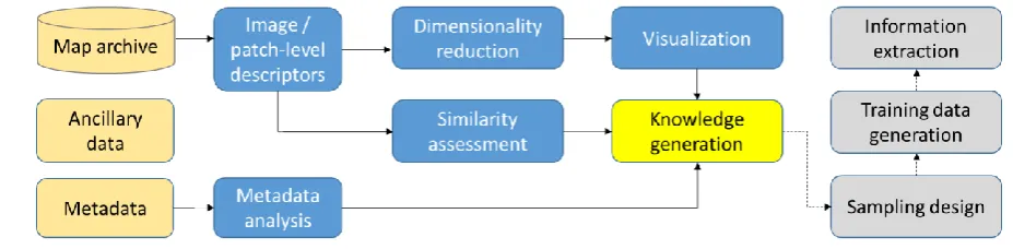
methods based on large map archives. Figure 3 shows how the proposed methods can be
208
incorporated in information extraction workflows.
209
210
211
Figure 3. The methodology for metadata analysis and content-based knowledge generation on map
212
archives to facilitate information extraction.
213
214
215
6 of 17
2.1.1. Metadata-based spatial-temporal coverage analysis
217
First, the temporal coverage of the map archives is analyzed. For the USGS map archive, which
218
is accompanied by structured metadata (i.e., text files including unique identifiers for each map
219
document), histograms based on the map reference year are created (Figure 4). It can be seen that the
220
peak of map production was in California in the 1950s, and slightly later, in the 1960s in Colorado.
221
(a) (b)
Figure 4. Histograms of USGS topographic maps (all available map scales) by reference year, (a) in
222
California, and (b) in Colorado (USA).
223
In addition to that, map production over time can be assessed in strata of map scales shown
224
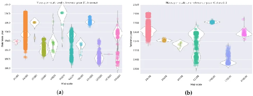
herein for the states of California and Colorado (Figure 5). These plots show the temporal distribution
225
of published map editions (represented by the dots) and give an estimate of the underlying
226
probability density (represented by the white areas) that indicates the map production intensity over
227
time, separate and relative for each map scale. Such a representation helps to understand which time
228
span can be covered with maps of various scales and thus can be used to determine which products
229
to focus on for a particular purpose. This is important because maps of different scale contain
230
different levels of detail resulting from cartographic generalization.
231
232
(a) (b)
Figure 5. Produced USGS topographic maps per reference year and map scale (a) in California, and
233
(b) in Colorado (USA).
234
In order to assess the spatial variability of map availability in a map archive over time, spatial map
235
footprints (i.e., delineating map quadrangles) are generated based on USGS-delivered metadata. For
236
each map footprint, statistics about available map sheets at those locations are computed. This allows
237
the spatial visualization of the number of map editions and the earliest reference year available for
238
each location, as shown in Figure 6 for the state of Colorado (scale 1:24,000), and for the map scales
239
representations are useful to identify regions that have been mapped more intensively versus those
241
for which temporal coverage is rather sparse. Furthermore, a user is immediately informed about the
242
earliest map sheets for a location of interest to understand the maximum time period covered by
243
these cartographic documents. Similar representations could be created for the average number of
244
years between editions or the time span covered by map editions of a given map scale.
245
(a) (b)
Figure 6. (a) Map edition counts and (b) earliest map production year per 1:24,000 map quadrangle
246
in the state of Colorado (USA) based on metadata analysis.
247
248
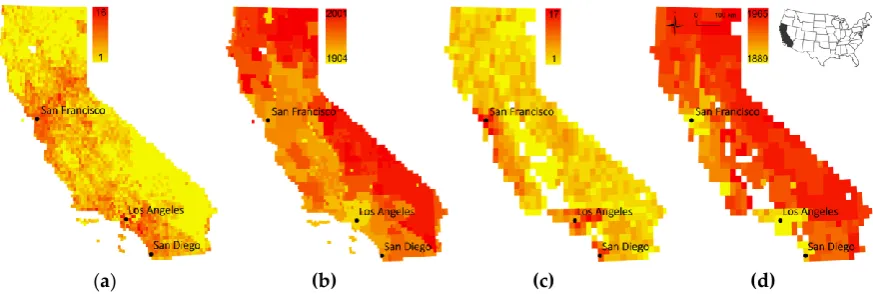
(a) (b) (c) (d)
Figure 7. (a) Map edition counts and (b) earliest map production year per 1:24,000 map quadrangle,
249
(c) map edition counts and (d) earliest map production year per 1:62,500 map quadrangle in the state
250
of California (USA) based on metadata analysis.
251
As a second example, the spatial-temporal coverage of the Sanborn fire insurance map archive
252
is visualized. Since Sanborn map documents are commonly not offered as georeferenced datasets,
253
this analysis is based on automatically extracted map locations (i.e., town or city name, county, and
254
state) that were collected from unstructured metadata retrieved from HTML-based web content of
255
the U.S. Library of Congress [45]. Additionally, the number of map sheets and their temporal
256
coverage per location are extracted. The extracted data are geocoded using web-based geocoding
257
services, which allows to visualize data availability and spatio-temporal coverage of Sanborn map
258
documents. Figure 8 shows, similar to the above examples, the year of the first map production and
259
the number of maps produced in total per location. The comparison of these visualizations for the
260
highlighted states of California and Colorado to the previously shown Figures 6 and 7 shows the
261
differences in spatio-temporal coverage between the two map archives, indicating a much sparser
262
spatial coverage of the Sanborn map archive, but extending further back in time than the USGS map
263
archive.
264
8 of 17
(a) (b)
Figure 8. Sanborn fire insurance map archive coverage: (a) year of first map production per location
266
and (b) number of available map sheets per location, both aggregated to grid cells of 10km for efficient
267
visualization. Highlighted in blue the states of California and Colorado for comparison to the USGS
268
map coverage shown in previous figures.
269
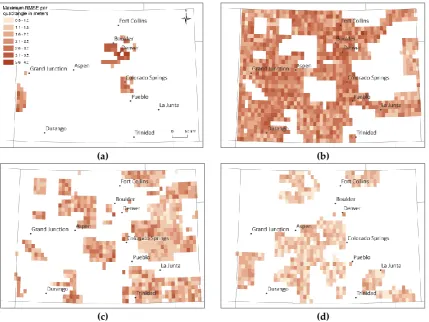
2.1.2. Metadata-based spatial-temporal analysis of positional accuracy
270
Positional accuracy of scanned maps can be caused by several factors, such as paper map
271
distortions due to heat or humidity, the quality of surveying measurements on which the map
272
production is based, deviations from the local geodetic datum at data acquisition time, cartographic
273
generalization, and distortions introduced during the scanning and georeferencing process. While
274
most of these effects cannot be reconstructed or quantified in detail, metadata delivered with the
275
USGS topographic map archive contains information about the ground control points (GCPs) used
276
for georeferencing the scanned map documents that allow for a partial assessment of these distortions
277
and resulting positional inaccuracies.
278
The USGS topographic map quadrangle boundaries represent a graticule. For example, the
279
corner coordinates for quadrangles of scale 1:24,000 are spaced in a regular grid of 7.5’x7.5’.
280
Additionally, a finer graticule of 2.5’x2.5’ is depicted in the maps. The intersections of this fine
281
graticule are used by the USGS to georeference the maps. Therefore, pixel coordinates at those
282
locations (i.e., the GCPs) are collected, and the corresponding known world coordinates of the
283
graticule intersections are used to establish a second-order polynomial transformation based on
least-284
squares adjustment. This transformation is used to warp the scanned document into a georeferenced
285
raster dataset. The GCP coordinate pairs are reported in the metadata, as well as an error estimate
286
per GCP that provides information on the georeference accuracy in pixels. Based on these error
287
estimates given in pixel units and the spatial resolution of the georeferenced raster given in meters,
288
the root mean standard error (RMSE) reflecting georeference accuracy in meters is calculated.
289
Appending these RMSE values as attributes to the map quadrangle polygons allows to visualize
290
georeferenced accuracy across the spatial-temporal domain. This is shown for the USGS maps of scale
291
1:24,000 in the state of Colorado (Figure 9) for different time periods, visualizing the maximum RMSE
292
per quadrangle and time period. Such temporally stratified representations are useful to examine if
293
the georeference accuracy is constant over time. It can be seen that the earlier years in this example
294
show higher degrees of inaccuracy than more recent map sheets. This has important implications for
295
the user who is interested in using maps from different points in time that may exhibit different levels
296
of inaccuracy.
297
(a) (b)
(c) (d)
Figure 9. Spatio-temporal patterns of georeference accuracy of USGS topographic maps (1:24,000) in
299
the state of Colorado (USA), for maps produced between (a) 1930-1950, (b) 1950-1970, (c) 1970-1990,
300
and (d) 1990-2004.
301
Besides this information, the distortion introduced to the map by the warping process can be
302
characterized by displacement vectors computed between the known world coordinates of each GCP
303
(i.e., the graticule intersections) and the world coordinates corresponding to the respective pixel
304
coordinates after applying the second-order polynomial transformation. These displacement vectors
305
reflect geometric distortions and positional inaccuracy in the original map (i.e., prior to the
306
georeferencing process) but are also affected by additional distortions introduced during
307
georeferencing inaccuracies or through scanner miscalibration.
308
Assuming that objects in the map are affected by the same degree of inaccuracy like the graticule
309
intersections, the magnitudes of these displacement vectors allow to estimate the maximum
310
displacements to be expected between objects in the map and their real-world counterparts that may
311
not be corrected by the second order polynomial transformation.
312
Figure 10 shows examples of these displacement vectors visualized for individual USGS map
313
sheets at scale 1:24,000 from Venice (California) produced in 1923, 1957, and 1975. The magnitude of
314
the local displacement is represented by the dot area, whereas the arrow indicates the displacement
315
angle. This example shows similar patterns across the three maps, probably reflecting
non-316
independent distortions between the maps since earlier maps are typically used as base maps for
317
subsequent map editions, and some local variations due to inaccuracies introduced during
318
10 of 17
320
(a) (b) (c)
Figure 10. Displacement vectors at GCP locations characterizing the distortions introduced during
321
the georeferencing of USGS topographic maps from Venice (California), produced in (a) 1923, (b) in
322
1957, and (c) in 1975 (from left to right).
323
Additionally, these displacement vectors can be visualized as vector fields across large areas,
324
allowing to identify regions, quadrangles, or individual maps of high or low positional reliability,
325
respectively. Figure 11 shows the vector field of relative displacements for USGS maps of scale
326
1:24,000 for a region Northwest of Denver, Colorado. Notable are the large displacement vectors in
327
the Parshall quadrangle, indicating some anomalous map distortion, whereas the Cabin Creek
328
quadrangle (Northeast of Parshall) seems to have suffered from very slight distortions only. Multiple
329
arrows indicate the availability of multiple map editions in given quadrangles. Such visualizations
330
may inform map users about the heterogeneity in distortions applied to the map sheets during the
331
georeferencing process and may indicate different degrees of positional accuracy across a given study
332
area.
333
334
335
Figure 11. Displacement vector field at GCP locations over multiple USGS map quadrangles of scale
336
1:24,000, located North-west of Denver (Colorado), reflecting different types of distortions introduced
337
to the map documents during the georeferencing process (Basemap source: [46]).
338
2.2. Content-based analysis
339
The presented metadata-based analysis provides valuable insights of spatial-temporal map
340
availability, coverage, and spatial accuracy without analyzing the actual content of the map archives.
341
However, it is important to inform the analyst about the degree of heterogeneity at content-level. In
342
based on low-level image descriptors computed for each map or map patches. Here, we employ
color-344
histogram based moments (i.e., mean, standard deviation, skewness and kurtosis, see [47]) computed
345
for each image channel in the RGB color space. Mean and standard deviation characterize hue,
346
brightness and contrast level of an image, skewness and kurtosis indicate the symmetry and flatness
347
of the probability density of the color distributions, and thus reflect color spread and variability of an
348
image. These four measures are computed for each channel of an image and stacked together to a
12-349
dimensional feature descriptor, at image or patch level. In the case of scanned map documents, such
350
descriptors allow to retrieve maps or patches of maps of similar background color (depending on
351
paper type and scan contrast level), and maps of similar dominant map content, such as waterbodies,
352
urban areas, or forest cover. This similarity assessment is based on distances in the descriptor feature
353
space and can involve metadata (e.g., map reference year), or ancillary geospatial data, to assess map
354
content similarity across or within different geographic settings. Furthermore, approaches for
355
dimensionality reduction such as t-distributed stochastic neighborhood embedding (t-SNE, [48]) are
356
employed to visualize the data based on similarity in feature space. T-SNE allows to reduce the
357
dimensionality of high-dimensional data, where the relative distances between the data points in the
358
reduced feature space reflect the similarity of the data points in the original feature space. This
359
facilitates the visual or quantitative identification of clusters of similar map sheets and provides a
360
better understanding of the content of large map archives and their inherent variability. This kind of
361
similarity assessment and metadata analysis is useful in generating knowledge which can be used to
362
guide sampling designs to generate template or training data for supervised information extraction
363
techniques.
364
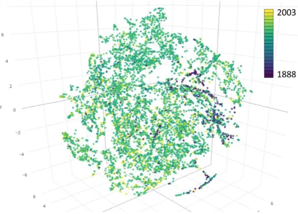
2.2.1. Content-based analysis at map level
365
Analyzing the content of the entire map archive with respect to similarities between the
366
individual map sheets is done by computing the image-moments based map descriptors. These
12-367
dimensional features are transformed into a reduced 3-dimensional feature space that can be
368
visualized and interpreted intuitively. Figure 12 shows the 3D feature space for the 6,964 USGS maps
369
in the state of Colorado. The map reference year is used to color-code the points representing
370
individual map sheets. The clusters of dark blue points indicate fundamentally different color
371
characteristics of old maps in comparison to more recent maps represented by points colored in
372
green-yellow tones.
373
374
Figure 12. T-SNE visualization of the 6,964 USGS maps in the state of Colorado in a 3D feature space
375
based on 12-dimensional image descriptors obtained from channel-wise image moments.
376
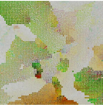
In addition to color-coding the data points by the corresponding map reference year, the
12-377
12 of 17
of individual maps corresponding to each data point in Figure 12. This transformation results in an
379
integrated visual assessment of map archives containing large numbers of map sheets. Figure 13
380
shows a t-SNE thumbnail visualization of a random sample (N=4,356) of the Colorado USGS maps in
381
a 2D feature space. Nearest neighbor snapping is used to create a rectified visualization. This is a very
382
effective way to visualize the variability in map contents, such as dominating forest area proportions.
383
It also illustrates the presence and abundance of different map designs and base color use, e.g., high
384
contrast and saturation levels in recent maps, compared to yellow-tainted map sheets from the
385
beginning of the 20th century centered at the bottom. The latter corresponds to the cluster of historical
386
maps located at the bottom of the point cloud in Figure 12.
387
388
389
Figure 13. Thumbnail-based visualization of a subset of the USGS topographic maps in the state of
390
Colorado (USA) based on a 2D transformation of the 12-dimensional image descriptor feature space
391
using t-SNE.
392
2.2.2. Content-based analysis at within-map patch level
393
In order to assess the content within map sheets, map documents can be partitioned into tiles of
394
a fixed size (exemplified here for 100x100 pixels). Low-level descriptors based on image moments can
395
then be computed for each individual patch. However, if the patch size is chosen small enough, it is
396
values in the patch) as a basis for t-SNE transformations. This can be useful if it is desired to introduce
398
a higher degree of spatiality and even directionality when assessing the similarity between the
399
patches. This method allows, for example, to rearrange a map document in patches based on patch
400
similarity, as shown for an example USGS map in Figure 14a. Quadrangle boundaries based on corner
401
coordinates delivered in the metadata can be used to clip the map contents and remove
non-402
geographic content in the map sheet edges. The clipped map content is then partitioned in tiles
down-403
sampled by factor 4, which results in a 1,875-dimensional feature vector per patch. These features are
404
then transformed into a 2D-space using t-SNE in order to create a similarity-based rearrangement of
405
the map patches (Figure 14b). This rearrangement highlights for example the groups of linear objects
406
of different dominant directions, such as road objects, or clusters of patches that contain contour lines
407
with diffuse directional characteristics. The incorporation of directionality may be useful to design
408
sampling schemes that generate training data allowing for rotation-invariant feature learning.
409
410
(a) (b)
Figure 14. (a) USGS topographic map for Boulder, Colorado (1966), and (b) rearranged map patches
411
according to their similarity in a raw pixel value feature space using t-SNE.
412
2.2.3. Content-based analysis at cross-map patch level
413
If variations of specific cartographic symbols across large map archives are of interest and have to be
414
characterized, ancillary geospatial data can be employed to label the created map patches based on
415
their spatial relationships to the ancillary data. For example, it may be important to assess the
416
differences in cartographic representations of dense urban settlement areas across map sheets, in
417
order to design a recognition model for urban settlement. In such situations building footprint data
418
with built-year information and the respective spatio-temporal coverage can be employed to
419
reconstruct settlement distributions in a given map reference year (see [49]). Based on these reference
420
locations, building density surfaces can be computed for each map reference year. Using appropriate
421
thresholding allows to approximately delineate dense settlement areas for a given point in time.
422
Based on spatial overlap between map patches and these dense reference settlement areas, map
423
patches that are likely to contain urban area symbols can be identified across multiple maps. These
424
selected map patches can then be visualized in an integrated manner using t-SNE arrangement, as
425
exemplarily shown in Figure 15 for map patches collected across 50 USGS maps (1:24,000) in the states
426
of Colorado and California. This arrangement illustrates nicely the different cartographic styles that
427
are used to represent dense urban settlements across time and map sheets, and provides valuable
428
14 of 17
locations where no ancillary data is available, and their content can be estimated based on descriptor
430
similarity (i.e., patches of low Euclidean distance in the descriptor feature space) or using
431
unsupervised or supervised classification methods.
432
433
Figure 15. T-SNE arrangement of cross-map samples of patches likely to contain dense urban
434
settlement symbols.
435
3. Conclusions and Outlook
436
In this contribution we propose a set of methods for systematic information mining and content
437
retrieval in large collections of cartographic documents, such as topographic map archives. These
438
methods consist of pure metadata-based analyses, as well as content-based analyses using low-level
439
image descriptors such as histogram-based color moments, and dimensionality reduction methods
440
(i.e., t-SNE). We illustrate the proposed approach by exemplary analyses of the USGS topographic
441
map archive and the Sanborn fire insurance map collection. Our approach can be used to explore and
442
compare spatio-temporal coverage of these archives, the variability of positional accuracy, and
443
differences in content of the map documents based on visual-analytical tools. These content-based
444
map mining methods are inspired by image information mining systems implemented for remote
445
sensing data archives and have been applied to facilitate the design and implementation of
446
information extraction methods [27,28] Further work will include the identification of suitable
447
textural measures to be incorporated in the image descriptors. Additionally, the benefit of map
448
archive indexing based on low-level image descriptors will be tested in a prototypic map mining
449
framework. Moreover, these efforts will contribute to the design of adequate sampling methods to
450
generate representative training data for large-scale information extraction methods from historical
451
map archives.
452
Acknowledgments: This material is based on research sponsored in part by the National Science Foundation
453
under Grant Nos. IIS 1563933 (to the University of Colorado at Boulder) and IIS 1564164 (to the University of
454
Southern California).
455
Author Contributions: J.H.U. and S.L. conceived and designed the experiments; J.H.U. performed the
456
experiments; J.H.U. analyzed the data; J.H.U. wrote the paper.
457
References
459
1. Chiang, Y.-Y.; Leyk, S.; Knoblock, C.A. A survey of digital map processing techniques. ACM Computing
460
Surveys 2014, 47, 1-44. http://dx.doi.org/10.1145/2557423
461
2. Miyoshi, T.; Weiqing, L.; Kaneda, K.; Yamashita, H.; Nakamae, E. Automatic extraction of buildings
462
utilizing geometric features of a scanned topographic map. In Proceedings of the 17th International Conference
463
on Pattern Recognition, 2004. ICPR 2004., IEEE: 2004. http://dx.doi.org/10.1109/icpr.2004.1334607
464
3. Laycock, S.D.; Brown, P.G.; Laycock, R.G.; Day, A.M. Aligning archive maps and extracting footprints for
465
analysis of historic urban environments. Computers & Graphics 2011, 35, 242-249.
466
http://dx.doi.org/10.1016/j.cag.2011.01.002
467
4. Arteaga, M.G. Historical map polygon and feature extractor. In Proceedings of the 1st ACM SIGSPATIAL
468
International Workshop on MapInteraction - MapInteract '13, ACM Press: 2013.
469
http://dx.doi.org/10.1145/2534931.2534932
470
5. Chiang, Y.-Y.; Leyk, S.; Knoblock, C.A. Efficient and robust graphics recognition from historical maps. In
471
Graphics Recognition. New Trends and Challenges, Springer Berlin Heidelberg: 2013; pp 25-35.
472
http://dx.doi.org/10.1007/978-3-642-36824-0_3
473
6. Miao, Q.; Liu, T.; Song, J.; Gong, M.; Yang, Y. Guided superpixel method for topographic map processing.
474
IEEE Transactions on Geoscience and Remote Sensing 2016, 54, 6265-6279.
475
http://dx.doi.org/10.1109/tgrs.2016.2567481
476
7. Leyk, S.; Boesch, R. Extracting composite cartographic area features in low-quality maps. Cartography and
477
Geographic Information Science 2009, 36, 71-79. http://dx.doi.org/10.1559/152304009787340115
478
8. Chiang, Y.-Y.; Moghaddam, S.; Gupta, S.; Fernandes, R.; Knoblock, C.A. From map images to geographic
479
names. In Proceedings of the 22nd ACM SIGSPATIAL International Conference on Advances in Geographic
480
Information Systems - SIGSPATIAL '14, ACM Press: 2014. http://dx.doi.org/10.1145/2666310.2666374
481
9. Chiang, Y.-Y.; Leyk, S.; Honarvar Nazari, N.; Moghaddam, S.; Tan, T.X. Assessing the impact of graphical
482
quality on automatic text recognition in digital maps. Computers & Geosciences 2016, 93, 21-35.
483
http://dx.doi.org/10.1016/j.cageo.2016.04.013
484
10. Tsorlini, A.; Iosifescu, I. ; Iosifescu, C. ; Hurni, L. A methodological framework for analyzing digitally
485
historical maps using data from different sources through an online interactive platform. e-Perimetron, 2014,
486
9(4), 153-165.
487
11. Hurni, L. ; Lorenz, C. ; Oleggini, L. Cartographic reconstruction of historic settlement development by
488
means of modern geo-data. Proceedings of the 26th International cartographic conference. Dresden,
489
Germany, 2013.
490
12. Leyk, S.; and Chiang, Y. Information extraction of hydrographic features from historical map archives using
491
the concept of geographic context. Proceedings of AutoCarto 2016, Albuquerque, New Mexico, USA, 2016.
492
13. Iosifescu, I.; Tsorlini, A. ; Hurni, L. Towards a comprehensive methodology for automatic vectorization of
493
raster historical maps. e-Perimetron 2016, 11(2), 57-76.
494
14. Budig, B.; van Dijk, T.C. Active learning for classifying template matches in historical maps. In Discovery
495
Science, Springer International Publishing: 2015; pp 33-47. http://dx.doi.org/10.1007/978-3-319-24282-8_5
496
15. Budig, B.; Dijk, T.C.V.; Wolff, A. Matching labels and markers in historical maps. ACM Transactions on
497
Spatial Algorithms and Systems 2016, 2, 1-24. http://dx.doi.org/10.1145/2994598
498
16. Budig, B.; van Dijk, T.C.; Feitsch, F.; Arteaga, M.G. Polygon consensus. In Proceedings of the 24th ACM
499
SIGSPATIAL International Conference on Advances in Geographic Information Systems - GIS '16, ACM
500
Press: 2016. http://dx.doi.org/10.1145/2996913.2996951
501
17. Maire, F.; Mejias, L.; Hodgson, A. A convolutional neural network for automatic analysis of aerial imagery.
502
In 2014 International Conference on Digital Image Computing: Techniques and Applications (DICTA), IEEE: 2014.
503
http://dx.doi.org/10.1109/dicta.2014.7008084
504
18. Castelluccio, M.; Poggi, G.; Sansone, C.; Verdoliva, L. Training convolutional neural networks for semantic
505
classification of remote sensing imagery. In 2017 Joint Urban Remote Sensing Event (JURSE), IEEE: 2017.
506
http://dx.doi.org/10.1109/jurse.2017.7924535
507
19. Audebert, N.; Le Saux, B.; Lefèvre, S. Semantic segmentation of earth observation data using multimodal
508
and multi-scale deep networks. In Computer Vision – ACCV 2016, Springer International Publishing: 2017;
509
16 of 17
20. Marmanis, D.; Datcu, M.; Esch, T.; Stilla, U. Deep learning earth observation classification using imagenet
511
pretrained networks. IEEE Geoscience and Remote Sensing Letters 2016, 13, 105-109.
512
http://dx.doi.org/10.1109/lgrs.2015.2499239
513
21. Romero, A.; Gatta, C.; Camps-Valls, G. Unsupervised deep feature extraction for remote sensing image
514
classification. IEEE Transactions on Geoscience and Remote Sensing 2016, 54, 1349-1362.
515
http://dx.doi.org/10.1109/tgrs.2015.2478379
516
22. Scott, G.J.; England, M.R.; Starms, W.A.; Marcum, R.A.; Davis, C.H. Training deep convolutional neural
517
networks for land–cover classification of high-resolution imagery. IEEE Geoscience and Remote Sensing
518
Letters 2017, 14, 549-553. http://dx.doi.org/10.1109/lgrs.2017.2657778
519
23. Zhao, W.; Jiao, L.; Ma, W.; Zhao, J.; Zhao, J.; Liu, H.; Cao, X.; Yang, S. Superpixel-based multiple local cnn
520
for panchromatic and multispectral image classification. IEEE Transactions on Geoscience and Remote Sensing
521
2017, 55, 4141-4156. http://dx.doi.org/10.1109/tgrs.2017.2689018
522
24. Zhang, L.; Zhang, L.; Du, B. Deep learning for remote sensing data: A technical tutorial on the state of the
523
art. IEEE Geoscience and Remote Sensing Magazine 2016, 4, 22-40. http://dx.doi.org/10.1109/mgrs.2016.2540798
524
25. Zhu, X.X.; Tuia, D.; Mou, L.; Xia, G.-S.; Zhang, L.; Xu, F.; Fraundorfer, F. Deep learning in remote sensing:
525
A comprehensive review and list of resources. IEEE Geoscience and Remote Sensing Magazine 2017, 5, 8-36.
526
http://dx.doi.org/10.1109/mgrs.2017.2762307
527
26. Ball, J.E.; Anderson, D.T.; Chan, C.S. Comprehensive survey of deep learning in remote sensing: Theories,
528
tools, and challenges for the community. Journal of Applied Remote Sensing 2017, 11, 1.
529
http://dx.doi.org/10.1117/1.jrs.11.042609
530
27. Uhl, J.H.; Leyk, S.; Yao-Yi, C.; Weiwei, D.; Knoblock, C.A. Extracting human settlement footprint from
531
historical topographic map series using context-based machine learning. In 8th International Conference of
532
Pattern Recognition Systems (ICPRS 2017), Institution of Engineering and Technology: 2017.
533
http://dx.doi.org/10.1049/cp.2017.0144
534
28. Uhl, J.H.; Leyk, S.; Yao-Yi, C.; Weiwei, D.; Knoblock, C.A. Spatializing uncertainty in image segmentation
535
using weakly supervised convolutional neural networks: a case study from historical map processing
536
(under review)
537
29. Duan, W.; Chiang, Y.-Y.; Knoblock, C.A.; Jain, V.; Feldman, D.; Uhl, J.H.; Leyk, S. Automatic alignment of
538
geographic features in contemporary vector data and historical maps. In Proceedings of the 1st Workshop on
539
Artificial Intelligence and Deep Learning for Geographic Knowledge Discovery - GeoAI '17, ACM Press: 2017.
540
http://dx.doi.org/10.1145/3149808.3149816
541
30. Duan, W.; Chiang, Y.-Y.; Knoblock, C.A.; Uhl, J.H.; Leyk, S. Automatic generation of precisely delineated
542
geographic features from georeferenced historical maps using deep learning (under review)
543
31. Fishburn, K.A.; Davis, L.R.; Allord, G.J. Scanning and georeferencing historical usgs quadrangles. In Fact
544
Sheet, US Geological Survey: 2017. http://dx.doi.org/10.3133/fs20173048
545
32. U.S. Library of Congress. Available online: http://www.loc.gov/rr/geogmap/sanborn/san6.html (accessed
546
on 28/02/2018).
547
33. U.S. Library of Congress. Available online: http://www.loc.gov/rr/geogmap/sanborn/ (accessed on
548
28/02/2018).
549
34. U.S. Library of Congress. Available online:
https://www.loc.gov/item/prn-17-074/sanborn-fire-insurance-550
maps-now-online/2017-05-25/ accessed on 28/02/2018).
551
35. National Library of Scotland. Available online: https://maps.nls.uk/os/index.html (accessed on 28/02/2018).
552
36. National Library of Scotland. Available online: http://maps.nls.uk/geo/explore (accessed on 28/02/2018).
553
37. Datcu, M.; Daschiel, H.; Pelizzari, A.; Quartulli, M.; Galoppo, A.; Colapicchioni, A.; Pastori, M.; Seidel, K.;
554
Marchetti, P.G.; D'Elia, S. Information mining in remote sensing image archives: System concepts. IEEE
555
Transactions on Geoscience and Remote Sensing 2003, 41, 2923-2936. http://dx.doi.org/10.1109/tgrs.2003.817197
556
38. Quartulli, M.; G. Olaizola, I. A review of eo image information mining. ISPRS Journal of Photogrammetry and
557
Remote Sensing 2013, 75, 11-28. http://dx.doi.org/10.1016/j.isprsjprs.2012.09.010
558
39. Espinoza-Molina, D.; Alonso, K.; Datcu, M. Visual data mining for feature space exploration using in-situ
559
data. In 2016 IEEE International Geoscience and Remote Sensing Symposium (IGARSS), IEEE: 2016.
560
http://dx.doi.org/10.1109/igarss.2016.7730543
561
40. Espinoza Molina, D.; Datcu, M. Data mining and knowledge discovery tools for exploiting big
earth-562
observation data. ISPRS - International Archives of the Photogrammetry, Remote Sensing and Spatial Information
563
41. Griparis, A.; Faur, D.; Datcu, M. Dimensionality reduction for visual data mining of earth observation
565
archives. IEEE Geoscience and Remote Sensing Letters 2016, 13, 1701-1705.
566
http://dx.doi.org/10.1109/lgrs.2016.2604919
567
42. Durbha, S.S.; King, R.L. Semantics-enabled framework for knowledge discovery from earth observation
568
data archives. IEEE Transactions on Geoscience and Remote Sensing 2005, 43, 2563-2572.
569
http://dx.doi.org/10.1109/tgrs.2005.847908
570
43. Kurte, K.R.; Durbha, S.S.; King, R.L.; Younan, N.H.; Vatsavai, R. Semantics-enabled framework for spatial
571
image information mining of linked earth observation data. IEEE Journal of Selected Topics in Applied Earth
572
Observations and Remote Sensing 2017, 10, 29-44. http://dx.doi.org/10.1109/jstars.2016.2547992
573
44. Silva, M.P.S.; Camara, G.; Souza, R.C.M.; Valeriano, D.M.; Escada, M.I.S. Mining patterns of change in
574
remote sensing image databases. In Fifth IEEE International Conference on Data Mining (ICDM'05), IEEE.
575
http://dx.doi.org/10.1109/icdm.2005.98
576
45. Library of Congress. Available online: http://www.loc.gov/rr/geogmap/sanborn/country.php?countryID=1
577
(accessed on 28/02/2018).
578
46. ESRI Basemaps: Esri, DigitalGlobe, GeoEye, Earthstar Geographics, CNES/Airbus DS, USDA, USGS, AEX,
579
Getmapping, Aerogrid, IGN, IGP, swisstopo, and the GIS User Community
580
47. Huang, Z.-C.; Chan, P.P.K.; Ng, W.W.Y.; Yeung, D.S. Content-based image retrieval using color moment
581
and gabor texture feature. In 2010 International Conference on Machine Learning and Cybernetics, IEEE: 2010.
582
http://dx.doi.org/10.1109/icmlc.2010.5580566
583
48. Van der Maaten, L; Hinton, G. Visualizing data using t-SNE. Journal of Machine Learning Research, 2008, 9,
584
2579-2605
585
49. Leyk, S.; Uhl, J.H.; Balk, D.; Jones, B. Assessing the accuracy of multi-temporal built-up land layers across
586
rural-urban trajectories in the united states. Remote Sensing of Environment 2018, 204, 898-917.