Article
1
Design and Implementation of a Programmable
2
Multi-Parametric Five Degrees of Freedom Seismic
3
Waves Geo-Mechanics Simulation IoT Platform
4
Hasan Tariq 1.*, Farid Touati 1, Mohammed Abdulla E. Al-Hitmi 1, Damiano Crescini 2 and Adel
5
Ben Mnaouer 3
6
1 Department of Electrical Engineering, College of Engineering, Qatar University, 2713, Doha, Qatar;
7
[email protected] (H.T.); [email protected] (F.T.); [email protected] (M.A.E.A.-H.)
8
2 Brescia University, 25121 Brescia, Italy; [email protected] (D.C.)
9
3 Canadian University Dubai, Dubai, UAE; [email protected](A.B.M.)
10
* Correspondence: [email protected]; Tel.: +974-50419852
11
Received: date; Accepted: date; Published:
12
Abstract: Natural calamities observation, study and simulation has always been a prime concern for
13
disaster management agencies. Billions of dollars are spent annually to explore geo-seismic
14
movements especially earthquakes but it has always been a unique accident. The real-time study of
15
seismic waves, ground motions, and earthquakes always needed a programmable mechanical
16
structure capable of physically producing the identical geo-seismic motions with seismology
17
domain definitions. A programmable multi-parametric five degrees of freedom electromechanical
18
seismic wave events simulation platform to study and experiment seismic waves and earthquakes
19
realization in the form of geo-mechanic ground motions is exhibited in this work. The proposed
20
platform was programmed and interfaced through an IoT cloud-based Web application. The
geo-21
mechanics was tested in the range of i) frequencies of extreme seismic waves from 0.1Hz to 178Hz;
22
ii) terrestrial inclinations from -10.000° to 10.000°; iii) velocities of 1km/s to 25km/s iv) variable arrival
23
times 1us to 3000ms; v) magnitudes M1.0 to M10.0 earthquake; vi) epi-central and hypo-central
24
distances of 290+ and 350+ kilometers. Wadati and triangulation methods have been used for entire
25
platform dynamics design and implementation as one of key contributions in this work. This
26
platform is as an enabler for a variety of applications such as training self-balancing and calibrating
27
seismic-resistant designs and structures in addition to studying and testing seismic detection
28
devices as well as motion detection sensors. Nevertheless, it serves as an adequate training colossus
29
for machine learning algorithms and event management expert systems.
30
Keywords: Motion sensors; seismic sensing; Wadati method; earthquakes; programmable;
31
simulation; test bench; calibration; machine learning; IoT platform.
32
33
1. Introduction
34
The natural disasters and accidents happen annually across the globe with earthquake and
35
floods being most devastating and alarming on the loss and damage benchmarks. The casualties
36
reported by natural calamities, i.e. 564.4million were the highest in 2006 as compared to the last 10
37
years [1], amounting to 1.5 times its annual average 224 million. The global natural disaster economic
38
damages, i.e. US$ 154 billion scrutinized in the last year as the fifth costliest since 2006, i.e. 12% above
39
the 2006-2015 annual average registered in CRED database. Earthquake or seismic events have
40
proven to be the most obvious and recurring in all [2] the natural disasters i.e. 14,568 in 2018. The
41
death toll of 2,256 on September 28, 2018 in Indonesia was at the top of charts.
42
Domain realization and perception assistance is the foremost constraint in all simulation
43
platforms design and implementations. In geo-seismic domain, a plethora of contributions were
44
observed in simulation area from theoretical and mathematical modelling aspect. The Tullis group
45
simulator RSQSim [3] was appreciable for fault-friction modelling, fully dynamic single-event
46
simulations, rate- and state dependent friction(RSF) modelling with a gap of wave modelling and
47
ground motions realization. The ALLCAL [4] was one of the earthquake simulators developed by
48
scientists of the Southern California Earthquake Center(SCEC) and belonged to Tullis group of
49
simulators. The ALLCAL used the Triangulation rule for the geometrical modelling and estimation
50
of stresses and displacement to approximate fault friction and elastodynamics at very abstract level
51
had a gap of mechanical implementation and core geo-seismic realization. The Viscoelastic
52
earthquake simulator for San Francisco Bay region [5] was very noticeable approach towards
53
seismicity functions with a gap of real surface motion kinematics, i.e. seismic waves and arrival times.
54
The Virtual Quake(VQ) earthquake simulator [6] was a simulation-based forecast of the El
Mayor-55
Cucapah region and evidence of predictability in simulated earthquake sequences was a successor of
56
Virtual California(VC) can be used for forecasting and training mechanics. The gap of physical design
57
and implementation was very prominent in VQ contribution. The physics-based earthquake
58
simulator replicated seismic hazard statistics across California [7] and compared its results with
59
UCERF3(Uniform California Earthquake Rupture Forecast, version 3) and RSQSim reliant on
60
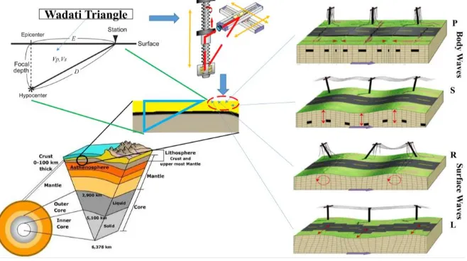
parameterized ground motion models(GMMs). The current state earthquake simulation [8]
61
contribution also had gaps in geo-seismic realization and its relationship with geo-mechanics
62
implementation. The gaps of geo-seismic realization as mechanical platform for physical
63
implementation were observed in all [3-8] contributions.
64
An effective early warning and disaster management(EWDM) needs a trustable ground motion
65
simulator for training and realization purposes. The contribution [9] was a generic earthquake test
66
and needed to be improved mechanically and electronically. The world’s largest ground motion
67
simulator(GMS) [10] was jointly owned by the Civil Defense College and Ankara Search & Rescue
68
Unit operated at 380V and delivered a maximum frequency of 12Hz and velocity of 80 cm/s needed
69
serious attention from the design of skeleton, power efficiency, and size. The second largest
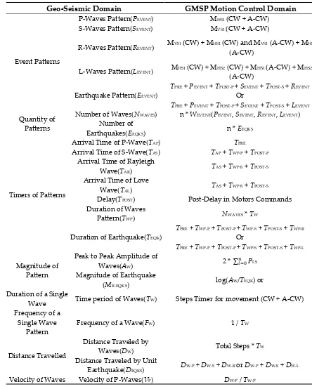
70
earthquake facility [11] in the world with a payload 1,200 tons, maximum velocity 200 cm/s, and
71
maximum displacement +/- 1 m for horizontal excitation and maximum velocity 70cm/s, maximum
72
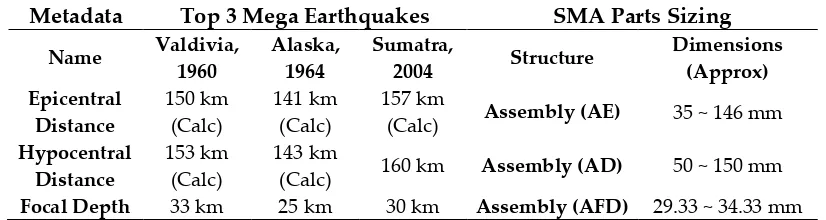
displacement +/- 50cm for vertical excitation to realize destructive ground motion was limited to a
73
shake table i.e. P-waves simulation needed improvement in design, mechanic, and electronics for
S-74
waves. The myQuake [12] was energy and payload optimized and had P-wave capabilities but
75
needed improvement in characteristic frequencies and amplitudes benchmarks. The seismic events
76
variable rotation test bench [13] with angular acceleration 2~500 rad/s, angular velocity 0.0002~35
77
rad/s, angular resolution 10:1700, frequency range 0.001~1000 Hz and payload 5kg needed
78
advancement in frequency, mechanical design, power economics, and IoT. The GG SCHIERLE [14]
79
shake table with spring-loaded mechanism and capable of vibration of 2.99Hz frequency and 3mm
80
amplitude needed rework and improvement in seismic definitions, drive electronics, mechanical
81
structure, IoT and results detailing. The State Key Laboratory for Disaster Reduction in Civil
82
Engineering, Tongji University had a reference shake table used in [15] with carrying capacity of 20kg
83
required seismic definitions, drive intelligence, wave parametric design, IoT and data set import
84
capabilities. The [16] shake table with motor shaft based motion control mechanism in UC, Berkley
85
needed IoT, web interface and data set import support features. The gaps of programmable
multi-86
parametric geo-seismic to geo-mechanics motion controls realization and integration in web interface
87
for remote simulation were observed all [3-16] contributions.
88
Dedicated and comprehensive efforts were observed in automation centered electro-mechanical
89
design full scale shake table [17] by NHERI Tall Wood Project Team with gaps in parameter settings
90
and upload from remote location and detailed programmable geo-mechanics control. The
91
programmability feature in Fuzzy-PLC based earthquake simulator [18] was a revolutionary add-on
92
but till gaps of geo-seismic realization to motion commands for motors as well as user-interface(UI)
93
as human machine interface(HMI) was the limitation. The multi-purpose earthquake simulator [19]
94
and a flexible development platform for actuator controller design had only P-wave simulation
95
capability was very basic design. The flexible IoT platforms [20-23] based design and implementation
96
efforts had very appreciable high-resolution bi-axial displacement, acceleration, and vibration
sensing capabilities and needed improvement in multi-parametric gap of mechanical actuation as
98
well as geo-seismic realization. The 4-DoF multi-parametric design [24] needed thorough
99
improvements in geo-seismic domain realization as well as IoT features [25] like web to actuator
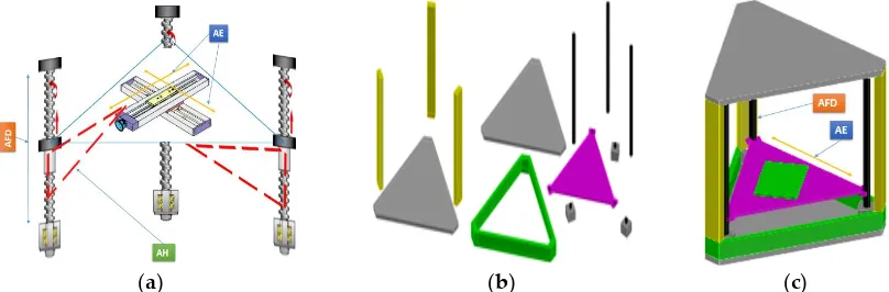
100
control accomplished in this work.
101
The nine target gaps that needed to be addressed were mechanical design in terms of, i) more
102
degrees of freedom(DOF); ii) multi-parametric geo-seismic realization; iii) geo-mechanics simulation
103
capabilities by motion control intelligence; iv) power efficiency; v) data sets upload and download
104
options; vii) web and IoT controls; viii) accuracy in P, S, Raleigh(R), and Love(L) waves; as well as ix)
105
customizable ground motions generation.
106
This work focuses on a complete programmable multi-parametric 5-DOF seismic wave ground
107
motions simulation platform (GMSP) for P, S, Rayleigh, and Love waves with the novel:
108
Multi-parametric Geo-Seismic Realization Engine(GRE) Design and Implementation
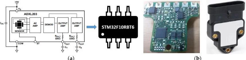
109
Programmable 5-DOF Seismic Machine Apparatus(SMA) Design and Fabrication
110
Motion Control System (MCS) or Mechatronics System Assembly and Programming
111
IoT Web Interface Design and Implementation with Seismic Parameters and Data Integration
112
2. GMSP Design and Implementation
113
A GMSP is a multi-sensing, multi-parametric, and programmable actuators platform that gives
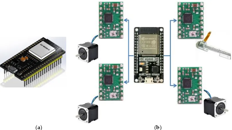
114
the exact realization of real seismic events by mathematical formulations. The first step is designing
115
any physical world simulation system is to realize the domain parameters. The second step is the
116
nearest possible physical model that resembles the real world application. In this third step, sensors
117
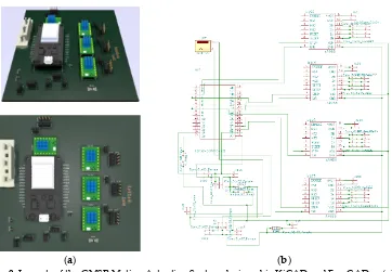
are selected that realize the domain variables. The fourth step is the flexibility or programmability of
118
actuators to create respective events. The entire conceptual model of this work in figure 1.
119
Figure 1. Overall Conceptual Layout of GMSP
2.1. Multi-parametric Geo-Seismic Realization Engine Design and Implementation
120
The objective of GRE was to convert seismological variables and parameters into actuator
121
commands and sense them to ensure the accuracy of the simulation system. In seismology, there are
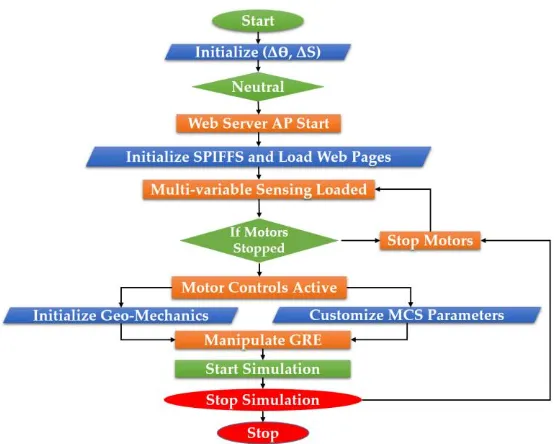
122
two basic types of waves i.e. body waves and surface waves with sub-types of each. Body waves have
123
two sub-types i.e. primary (P), secondary(S) and surface waves have Rayleigh(R) and Love(L) waves.
124
For a sensing system, seismic waves are very specific ground motion events that need to be sensed
125
in x, y, and z directions as DX, DY, and DZ. In figure 1, it can be observed that seismic waves study is
126
focused on ground motion and anomalies in lithosphere and crust only. The point where the seismic
127
fault occurs and generates the earthquake is called hypocenter(CH) and its perpendicular point on
128
earth surface is called epicenter(CE). The point where seismic variables are observed is called a seismic
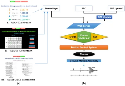
station(SS). The hypocenter and epicenter measurement assists in the computation of magnitude(M)
130
and energy(E) of earthquakes. After seismic motion generation, the triangulation method is used to
131
find the epicenter as the first step. Three seismic stations are a mandatory requirement for the
132
triangulation method. The P, S, R and L waves can be sensed any high-sampling and precision
bi-133
axial motion sensors. The waves velocity or motion needs accelerometers and angular displacement
134
needs inclinometers tactically oriented in x, y and z-axis. The conversion of seismic variables into
135
motion control commands in given below in Table I. Let the five motors be first horizontal shaft motor
136
be MHS1, second horizontal shaft motor be MHS2, first vertical shaft motor be MVS1, second vertical shaft
137
motor be MVS2, and third vertical shaft motor be MHV3.
138
Table 1. Realization Geo-Seismic Events as Motion Control Commands
139
Geo-Seismic Domain
GMSP Motion Control Domain
Event Patterns
P-Waves Pattern(PEVENT) MHS1 (CW + A-CW)
S-Waves Pattern(SEVENT) MVS1 (CW + A-CW)
R-Waves Pattern(REVENT) M
VS1 (CW) + MHS1 (CW) and MVS1 (A-CW) + MHS1
(A-CW)
L-Waves Pattern(LEVENT) M
HS1 (CW) + MHS2 (CW) + MHS1 (A-CW) + MHS2
(A-CW)
Earthquake Pattern(EEVENT)
TPRE + PEVENT + TPOST-P + SEVENT + TPOST-S + REVENT
Or
TPRE + PEVENT + TPOST-P + SEVENT + TPOST-S + LEVENT
Quantity of Patterns
Number of Waves(NWAVES) n * WEVENT(PEVENT, SEVENT, REVENT, LEVENT)
Number of
Earthquakes(EEQKS) n * E EQKS
Timers of Patterns
Arrival Time of P-Wave(TAP) TPRE
Arrival Time of S-Wave(TAS) TAP + TWP-P + TPOST-P
Arrival Time of Rayleigh
Wave(TAR) T
AS + TWP-S + TPOST-S
Arrival Time of Love
Wave(TAL) T
AS + TWP-S + TPOST-S
Delay(TPOST) Post-Delay in Motors Commands
Duration of Waves
Pattern(TWP) N
WAVES * TW
Duration of Earthquake(TEQK)
TPRE + TWP-P + TPOST-P + TWP-S + TPOST-S + TWP-R
Or
TPRE + TWP-P + TPOST-P + TWP-S + TPOST-S + TWP-L
Magnitude of Pattern
Peak to Peak Amplitude of
Waves(AW) 2 * ∑𝑛 𝑃
𝑖=0 LS
Magnitude of Earthquake
(MR-EQKS) log(A
W/TEQK) or
Duration of a Single
Wave Time period of Waves(TW) Steps Timer for movement (CW + A-CW) Frequency of a
Single Wave Pattern
Frequency of a Wave(FW) 1 / TW
Distance Travelled
Distance Traveled by
Waves(DW) Total Steps * T W
Distance Traveled by Unit
Earthquake(DEQKS) D
W-P + DW-S + DW-R or DW-P + DW-S + DW-L
(can be X and Y) Velocity of S-Waves(VS) DW-S / TW-S
Velocity of R-Waves(VR) DW-R / TW-R
Velocity of L-Waves(VL) DW-L / TW-L
Impact of P-Waves w.r.t to Equator and
Poles
Angle of Incidence P-Waves(ƟP)
(can be X and Y)
Average Angle of P-Cluster where angle and acceleration is similar
Impact of S-Waves w.r.t to Equator and
Poles
Angle of Incidence P-Waves(ƟS)
(can be X and Y)
Average Angle of S-Cluster where angle and acceleration is similar
Hypocenteral Distance
Hypotenuse of Wadati
Triangle (HWT) B
WT / {cos((ƟS+ ƟP)/2)}
Epicentral Distance Base of Wadati Triangle
(BWT) (T
AS - TAP) * {(VP* VS)/ (VP - VS)}
Epi-Hypo Distance Perpendicular of Wadati
Triangle (PWT) B
WT / {sin((ƟS+ ƟP)/2)}
Location of SS GPS Coordinates (Y°N, X°E) Longitude and Latitude Values
Location of (CH, CE) GPS Coordinates of Offset =
(BWT) from SS ((Y°N, X°E)
SS (Y°N, X°E) + (BWT [sin{(ƟS+ ƟP)/2}]°N, BWT
[cos{(ƟS+ ƟP)/2}]°E)
In table 1, all the information regarding GRE is given. Clockwise and anti-clockwise rotation is
140
expressed as CW and A-CW. Further details can be read from references cited in the introduction.
141
2.2. Programmable 5-DOF Seismic Machine Apparatus Design and Fabrication
142
The mechanics of seismic events and earth typography prevails the design of SMA
143
measurements and design constraints. The extreme values for seismic variables in top 3 earthquakes
144
i.e. the Chile Earthquake (1960) with M9.5, the Atlanta earthquake (1964) with M9.2 and the Indian
145
Ocean earthquake (2004) with M9.1 have been employed as standard design parameter set. The SMA
146
design process has been divided into two sections:
147
SMA Static Parts Sizing and Dimensions
148
SMA Dynamic Parts Sizing and Dimensions
149
2.2.1. SMA Static Parts Sizing and Dimensions
150
The epicenter, hypocenter, focal depth, triangulation area, and seismic station are the static
151
locations on the map thus their mechanical equivalents will also be static components. The global
152
datasets on IRIS and USGS were used to specify the limits and extent of parts designed and used for
153
mechanical structure. Considering into account the top 3 earthquakes i.e. 1960 Chilean earthquake in
154
Valdivia with Richter M9.5, 1964 Alaska earthquake with Richter M9.2~9.3 and 2004 Indian Ocean
155
earthquake in Sumatra with Richter M9.1, the static parts sizing was accomplished. The re-scaled
156
sizing was performed in the same ratios to streamline the dimensions of static parts in GMSP given
157
in table 2.
158
Table 2. GRE Dimensions for SMA Static Parts
159
Metadata
Top 3 Mega Earthquakes
SMA Parts Sizing
Name Valdivia, 1960
Alaska, 1964
Sumatra,
2004 Structure
Dimensions (Approx) Epicentral Distance 150 km (Calc) 141 km (Calc) 157 km
(Calc) Assembly (AE) 35 ~ 146 mm
Hypocentral Distance
153 km (Calc)
143 km
(Calc) 160 km Assembly (AD) 50 ~ 150 mm
Magnitude 9.5 9.2 9.1 Oscillation
Tolerance
Hinged Joint (MS + Acrylic)
Triangulation Area
10 km E 90 km W 120 km N
20 km N 125 km E 64 km W
Not
Found GMSP Bed (GB)
300mm Side A 300mm Side B 300mm Side C
The 3D models of SMA static parts were designed in AutoCAD and are shown in figure 2. The
160
word “(Calc)” means it was mathematically calculated using Pythagoras theorem and “Not Found”
161
means that we could not found any reliable source of information for this field. The dimensions are
162
approximated from the average of parameters of top 3 earthquakes.
163
(a) (b)
Figure 2. Core components of SMA Static Parts 3D Model as (a) GMSP Bed Dimensions; and (b) Assemblies (AE, AD, AFD)
In figure 2, it can be seen that initially static parts have been designed on the basis of realistic
164
approximation of geology of top 3 earthquakes with scaling ratio of 0.33mm = 1km means GMSP bed
165
is capable of simulating 1000km crust surface. The three corners represent 3 seismic stations in
166
accordance with the Wadati triangle method and triangulation rule for geo-seismic estimations.
167
2.2.2. SMA Dynamic Parts Sizing and Dimensions
168
The dynamic parts include gears, shafts; and motors. The seismic waves velocities, frequencies,
169
and wavelengths have led dynamic parts estimation. Considering into account of the standard
170
seismology literature referred in the introduction section, the dimensions of the dynamic parts are
171
given in table 3. The seismic velocities were governed by lead screws coupled with bi-polar stepper
172
motors, frequencies by rotation per second(RPM) of motors by full-stepping and micro-stepping and
173
wavelengths by the pitch of lead-screws and number of threads traveled per second. The unit pitch
174
was the minimum unit of velocity for any wave and half times of rated RPM stepper was expected
175
frequency generated by stepper motor as a multi-parametric actuator.
176
Table 3. GRE Dimensions for SMA Dynamic Parts
177
Metadata
Seismic Waves
SMA Parts Sizing
Parameters P S R L Structure Dimensions
Velocity 5~8 km/s 3~4 km/s 2~4.2 km/s 2~4.4 km/s Lead (TPS) 2~8
Frequency 4~8 Hz 1.5~3 Hz 0.03~0.7 Hz 0.05~0.5 Hz Motor(RPM/2) 16~32
Wavelength 5m~50 km 30m~500km 30 to 1000 km Length(Screws) 0.05~500mm
The frequencies have been achieved using revolution per minute, wavelength through the
178
amplitude of vibration by scaling radius of earth R = 6.371km i.e. circumference, C = 40,075 km. The
179
average of wavelength of P-wave, λP = 25km and S-wave, λS = 235km, diving it into least count of a
180
measurement instrument C/ λ = (1603, 170.5) means that for GMSP the minimum displacement for
P-181
wave is dP = 1.603cm and S-wave is, dS = 0.17cm to realize the comparative ground motions. For this,
two different lead screw assemblies were selected with stepper motors with step angles 1.8° and
183
5000RPM, 20 steps per revolution for P-wave to achieve dP and 200 steps per revolution for dS. The
184
desired assembly was designed in AutoCAD as 2D and 3D and given in fig 2 as a 4 DOF motion
185
platform. The considerations like epicenter and seismic center have been kept in account while
186
designing the mechanical assembly for GMSP.
187
Table 4. Stepper Motor and Lead Screw Specifications
188
Parts
Stepper Motors Specs
Lead Screws Dimensions
Motors RPM Steps Step-Angle Screws Pitch TPI Length Diameter Type 1 >32 200 1.8° Type 1 1.25mm 20 500mm 8mm
Type 2 >16 18 20° Type 2 3mm 8.5 140mm 3mm
Table 4 is complete interpretation and derivation from table 3, i.e. geo-seismic mechanics to the
189
electromechanical domain. The motors and lead screws parameters are computed by maximum
190
possible limits of high flexibility in the precision of the system.
191
(a) (b)
Figure 3. Description of SMA Dynamic Parts Mechanical CAD and 3D Model as (a) Lead Screws Design; and (b)Specifications Assemblies (AE, AD, AFD)
In figure 3, it can be seen that initially dynamic parts have been designed on the basis of realistic
192
approximation mechanics of seismic waves from IRIS and USGS database. The pitch 1.25mm assists
193
in 4km surface movement and 3mm in 9km as per scaling defined in table 3 i.e. single revolution of
194
type 1 motor created motion of 4km and type 2 motor created 9km i.e. at max RPM will produce
195
velocities of 1200km/min and 27000km/m. This speed is much more than realistic seismic velocities.
196
The overall assembly is given in figure 4.
197
(a) (b) (c)
Figure 4. Exhibition of Overall GMSP Assembly and 3D Model as (a) Internal Assembly; (b) Overall Parts 3D Model (c) Assembled GMSP
In figure 4, the internal assembly is scaled and oriented according to the triangulation and
198
Wadati method based on real-world calculations. The external assembly serves the purpose of
alignment and minimizing kinematic disturbances due to linear and angular motions and resulting
200
vibrations. The entire concept of GSMP is given in the figure below.
201
Figure 5. The Comprehensive Realization of GMSP
In figure 5, the overall system is defined with geo-seismic reference and its operation capacity
202
as a three station simulation platform as three equidistant assemblies (AE, AD, AFD) for A, B and C
203
geo-locations.
204
3. Motion Control System (MCS) or Mechatronics System Assembly and Programming
205
The GMSP MCS consists of three subsystems the seismic heterogeneous sensing node,
geo-206
seismic actuator-drive system and MCS controller with IoT enablement capabilities. The GMSO at
207
boot up is initialized with a perfectly static structure. The first step after booting is normalizing the
208
SMA to 0 tilt-angle and move the GB to origin so that there are no offsets by the help of
209
instrumentation support. In the second step, the GMSP gives an indication of “Ready” and is ready
210
to take user inputs. The three components of MCS are:
211
Geo-seismic heterogeneous-sensing node(GHN)
212
Geo-seismic mechanics actuators-drive system (GMAS)
213
GMSP MCS Controller
214
3.1. Geo-seismic heterogeneous-sensing node(GHN):
215
The block diagram of GHN is given in figure 6 focusing on the measurement requirements in
216
table 3. A bi-axial accelerometer ADXL203 has been used for heterogeneous sensing i.e. acceleration
217
and as well as tilt-angle measurements.
218
(a) (b)
In figure 6, the STM32F10RBT6 (32-Bit microcontroller with CAN-Open Transceiver and 12-Bit
219
ADC with a sampling rate of 1us) is interfaced with ADXL203 using to two ADC channels to
220
constitute one GHN as per (a) and PCB as wells as IP68 enclosure is displayed in (b).
221
3.2. Geo-seismic mechanics actuators-drive system (GMAS)
222
The bipolar stepper motors type1 and type2 specified in table 3 are shown in figure 7 with respective
223
motor drives i.e. A4988 with micro-stepping capabilities. The RPM and acceleration programming
224
was also a novel task performed in this work for geo-mechanics. The motion control system consists
225
of an ESP32 an Xtensa II 32-Bit SoC coupled with A4988 stepper drivers with micro-stepping
226
capabilities and 12V/2A power supply drive for bi-polar stepper motors. The overall system layout
227
is given in fig 3.
228
i. Bi-polar Stepper Motor (12V/0.5A)
ii. A4988 Motor Driver
iii. Bi-polar Stepper motor (12V/0.12A)
iv. A4988 Motor Driver
(a) (b)
Figure 7. The GMSP Motors and Drives as (a) Type 1 Motor Drive System; and (b) Type 2 Motor Drive System.
Three bi-polar type1 for vertical movements and 2 bi-polar type2 for horizontal motions were
229
used in GMSP.
230
(a) (b)
Figure 8. The GMSP Motion Actuation System as (a) Xtensa II 32-Bit SoC (ESP32); and (b) Motion Control System Layout.
In figure 8, it is prominent that a five joint system is powered using 5 stepper motors driven by
231
five A4988 stepper drivers controlled through a single ESP32.
(a) (b)
Figure 9. Layouts of the GMSP Motion Actuation System designed in KiCAD and FreeCAD as (a) PCB Layout Top Views (MCS); and (b) Motion Control System Schematics.
A complete GMAS MCS motherboard is shown that enables the entire GMSP is displayed in
233
figure 9. The 3D view of the PCB of the GMSP MCS motherboard is displayed in figure 9(a) and
234
detailed schematics in figure 9(b) sum up the contribution. Two further novelties in this work are
235
schematic symbols, PCB footprints designs, and integration of their 3D models designed in FreeCAD
236
with KiCAD footprint designer module.
237
3.3. GMSP MCS Controller
238
The GMSP MCS controller has three core components that are being used for overall GMSP:
239
SMA Orientation Neutralizer(SON).
240
SPIFFS (Serial Peripheral Flash File System) for a web interface for 3 pages.
241
GRE SSG (Seismic Sequence Generator) for OTA firmware.
242
The control algorithm of the GMSP MCS is given in figure 10. The GMSP MCS follows a
243
sequential methodology of operations given as:
244
1. When System is powered on it takes inputs from GHN and brings itself into zero “g”
245
condition i.e. removes all the initial value offsets using SON mechanism. Motors operate
246
till it's zero acceleration and displacement at 0° tilt.
247
2. After SON operations, the access point is created, then AP is created after the acquisition
248
of IP address. After a stable web server creation, the GMSP loads associated pages from
249
SPIFFS for its user interactive web interface explained in later sections.
250
3. The GRE is stored as a binary code in firmware of SoC and is ready to receive user
251
commands that simulate geo-mechanics by SMA actuated by MCS.
Figure 10. Flowchart of GMSP MCS Control Algorithm
Figure 10, the control algorithm of MCS and very self-explanatory from start till end. Safety
253
operation in MCS is very vital that is neutralizing and stopping the motors by feedback control from
254
GHN.
255
4. IoT Web Interface Design and Implementation with Seismic Parameters and Data Integration
256
The IoT web interface gives full flexibility in real-time geo-seismic sensing at the 100Hz sampling
257
frequency, seismic waves and earthquake simulation by GMSP actuation, customized geo-seismic
258
ground motion stimulus generation. HTML, CSS, and JavaScript were used to create user-friendly
259
interfaces comprised of 4 web pages stored in SPIFFS of SoC. The four unique pages have 4 unique
260
functions explained below:
261
Page 1: GHN Dashboard
262
Page 2: Geo-Seismic Mechanics Actuators-Drive System (GMAS) Workbench
263
Page 3: GMSP Motion Control System(MCS) Stimulus Dataset Generator
264
When the system boots it creates an access point where all the users can connect to access the
265
controls given on web named “NPRP8 Seismic Simulation Rig”.
266
The HTML and CSS component that is being used as a frontend for user interaction is stored in
267
SPIFFS and the main code with Web Server, AP, motor control instructions and wave generation
268
functions in C are stored as SSG. The Page 1 i.e. GHN dashboard it active all the time and is displaying
269
values as 100Hz refresh rate to inform the current state of X, Y tilt and acceleration. Page 2 has two
270
portions one is dedicated for stored seismic waves simulation and the second part is earthquake
271
simulation based on detailed data-set format required by GMSP that can be converted into motor
272
controls. The USGS and IRIS datasets have to first convert into GMSP format. The datasets found on
273
the cloud were having gaps and missing values. The extensive workout was required for the flawless
274
formulation of IRIS and USGS datasets to be made adaptive with GMSP operational parameters. Page
275
3 is geo-seismic domain based control form with all the parameter setting and simulation flexibility.
i. GHN Dashboard
ii. GMAS Workbench
iii. GMSP MCS Parameters
(a) (b)
Figure 11. Description of GMSP IoT Web Platform as (a) Demo Pages; and (b) IoT Web Flow Diagram.
The first step after booting is normalizing the SMA to 0° tilt-angle and move the GB to origin so
277
that there are no offsets by the help of instrumentation support. In the second step, the GMSP gives
278
an indication of “Ready” and is ready to take user inputs. The three pages of GMSP Web-based
279
hardware management system are:
280
5. Results and discussion
281
The GSMP was assembled for performing the experiments as shown in fig 6. The experiment
282
has been set up with a bi-axis accelerometer node with 14-bit resolution also designed and fabricated
283
in our previous works [13-15].
284
(a) (b)
The results were observed from three sources, i.e. the GHN dashboard, Tektronix TDS 2014
285
oscilloscope and MATLAB serial input. The GMSP results are very fertile and perceivable by
286
seismologists and geologists.
287
(a) (b)
Figure 13. IoT Web Interface of GMSP as (a) AP Mode for Web Server Access; and (b) Home Page of GMSP IoT Platform.
The first indication for user interaction is the visibility of AP in wireless networks as shown in
288
figure 13. After connecting to the AP the user needs to give IP of the gateway from network settings
289
in the URL text field of web browser i.e. 192.168.1.1:81. This opens the GHN dashboard with current
290
values. All the GHN values must be 0 to start the operation of GMSP.
291
Figure 14. IoT Web GHN Dashboard
The first page is the GHN dashboard page as shown in figure 14 with a refresh rate of 100Hz.
292
These values have to be almost zero to start the operation of GMSP. It needs a 10 to 20 min calibration
293
in the worst case as SMA neutralizer self-calibrates the GMSP bed to achieve zero offset condition.
294
The results were observed from two sources, i.e. the Tektronix oscilloscope and MATLAB serial
295
input. The GMSP results are very fertile and perceivable by seismologists and geologists.
Figure 15. IoT Web GMAS Workbench – Seismic Wave Simulation (Top section)
This is a static page i.e. Page 2 shown in figure 15. Just press web buttons and start operations.
297
The active operation button turned green. The P, S and surface waves are simulated just by pressing
298
buttons according to the given parameters in Page 3.
299
Figure 16. IoT Web GMAS Workbench – Earthquake Simulation (Bottom section)
The second section of Page 2 is shown in figure 16 i.e. dedicated for earthquake simulation. The
300
green color of a button means “No Datasets Loaded”. Upon loading the buttons became blue. One of
301
the key work in GMSP is designed a native IRIS and USGS dataset converter on a chip that can load
302
live data from the cloud and simulate it on the go.
Figure 17. IoT Web GMAS Workbench – Seismic Wave Simulation (Top section)
The customized parameters input for GMSP to create seismic waves as well as the earthquake
304
of any type that covers the safety and integrity of the motorized system as shown in figure 17. Page
305
3 creates a motor command file on SPIFFS that stays that there deleted. These values become the right
306
hand side variables of GRE.
307
(a) (b)
Figure 18. Observations of GMSP Simulation from Tektronix 2014 Oscilloscope as (a) P-Wave with 10.3mm Wavelength at 8 Hz; and (b) S-Wave with 17mm wavelength at 4 Hz.
The results on the oscilloscope are very self-explanatory where the yellow line is for x-axis or
308
vertical motion and cyan line for y-axis or horizontal motion. The frequencies achieved by the system
309
are almost ideal and very accurate as shown in figure 18. The P-wave crust and trough is very
310
extremely high and prominent with time period 100ms and unit segment of oscilloscope ±1.6VPK-PK
311
covers 80% of the x-axis as proof of 8Hz frequency in figure 18(a). The s-wave is being measured at
312
the same settings except that the unit division is 200mV i.e. total of 5 divisions on the y-axis and slight
313
variation of ±10mV on the x-axis in figure 18(b).
(a) (b)
Figure 19. Observations of GMSP Simulation observed from Tektronix 2014 Oscilloscope as (a) R-Wave with 16.03mm Wavelength at 35.73 Hz; and (b) L-Wave with 1.7mm wavelength at 78.092 Hz.
The results for R and L waves on the oscilloscope are very self-explanatory in figure 19. The
315
frequencies achieved by the system i.e. 35Hz+ and 78Hz+ are extremely high and show the capability
316
of the system to generate 10 times faster frequencies that were not observed in the literature before
317
for R and L waves. The value 3.57684kHz is due to motor internal vibration when overstepped and
318
accelerated to above final limits and creates plenty of pseudo-random noise that can be observed in
319
the signal.
320
A much detailed observation of figure 19 (a) shows that R wave motion is translating along
x-321
axis showing ±2.5 VPK-PK at 500mV grid setting i.e. slightly higher than the y-axis ±2.2 VPK-PK at 1V grid
322
setting. In figure 19 (b) its only z-axis motion by changing the orientation of GHN on GMSP bed i.e.
323
showing ±2.1 VPK-PK at 500mV grid setting. This surface motion is much challenging to produce as is
324
only in one axis rest axis contain noise only.
325
(a) (b)
(a) (d)
The GMSP generated different earthquakes by varying the frequency as well as the amplitude
326
of displacement as shown in figure 19. The characteristic earthquake pattern has used a masterpiece
327
for simulation and all the patterns shown in figure 20 from (a) to (b) are by studying different
data-328
sets mentioned in the literature review. The duration of an earthquake is 8s in figure 20 (a) i.e. 1s to
329
9s on scope, P-waves arrival after 2s, S-waves after 4s and surface waves after 6s. Two earthquakes
330
in figure (c) with duration 5.5 seconds without gap i.e. from 1.5s to 6s for first and 6s to 10s for the
331
second earthquake with a 100mV amplitude of P-wave, 320mV for S-wave and 505mV for surface
332
waves. The numbers 7.73085kHz, 88.6411kHz, and 89.6924kHz are due to pseudo-random noise
333
produced by stepper motors being a different research domain in electro-mechanical engineering.
334
The serial out of the ESP32 was connected to PC for observations in MATLAB. The results in
335
MATLAB were digital and had a lesser impact of pseudo-random noise observed in TDS 2014.
336
Figure 20. P-Waves observed in MATLAB for 8Hz on the x-axis
First, figure 18 (a) code was simulated and ±1.6VPK-PK curves were observed in MATLAB by only
337
considering the x-axis acceleration signal. The plot captured data trace shows a significant difference
338
in clarity in digital and analog data processing outputs.
339
Figure 21. S-Waves observed in MATLAB
Furthermore, figure 18 (b) code was simulated and ±2.2VPK-PK curves were observed in
340
MATLAB. The 200mV grid setting plot on the 2000ms scale on TDS 2014 displayed as figure 21 in
341
MATLAB as a 1000ms scale for y-axis signal to demonstrate vertical ground motion capabilities.
Figure 22. L-Waves observed in MATLAB at 1Hz
GMSP simulated L-wave with time period TL>1.1s can be observed in MATLAB for custom
343
parameters given in GMSP MCS stimulus page as shown in figure 22. The eight waves traveling over
344
the crust can be observed in figure 22. The gradual degradation or depreciation in amplitude and
345
time period of all the seismic waves is to seismic parameter Ψ dependent on the elasticity of and
346
density of medium or stress and strain bearing capacity of the medium. In this simulation Ψ = 6.21
347
has been used.
348
Figure 23. R-Waves observed in MATLAB
Figure 23 is based on R-wave simulation at Ψ = 6.21 and with the time period of TR = 1s. The
349
circles show the loading effect of motors and axis at a point where x-axis and y-axis motion merges
350
or maximum x-axis value for a given y-axis i.e. when y-axis displacement just about to converge or
351
touch the x-axis displacement its green and when axis about to diverge its purple means more
y-352
axis and less x-axis means anti-clockwise in both scenarios.
Figure 24. GMSP simulated Earthquake captured in MATLAB (4 seconds)
An earthquake comprised of eight P-waves of ±0.4VPK-PK amplitude and frequency 8Hz in the
x-354
axis, four S-waves with ±1VPK-PK amplitude and frequency 4 Hz in the y-axis, three L-waves with
355
±2.1VPK-PK amplitude in the y-axis and three R-waves with ±2.5VPK-PK amplitude in z-axis were
356
simulated based on standard earthquake seismograph.
357
6. Conclusions
358
A multi-parametric five degree-of-freedom seismic wave ground motions simulation platform
359
for P, S, L and R seismic waves was designed, fabricated, assembled, programmed and tested for
360
multiple ground motions i.e. at different frequencies, amplitudes, patterns, arrival times of seismic
361
events. The possible minima and maxima were tested and results show that GMSP can serve as a
362
reliable source for remote earthquake simulation and detection as global scale AI and machine
363
learning platform. The results show the significance of GMSP for geo-physicists especially
364
seismologists, a new era for motion control system developers, virtual reality and augmented reality
365
scientists and data scientists to test their datasets. The platform was successful in emulating standard
366
as well as extreme ranges of seismic frequencies, displacements, and velocities at given seismic
367
parameters in addition to possible theoretical estimations in geo-seismic systems. Architects and
368
construction engineers can use this platform to improve their realization for seismic-tolerant design
369
and advise better structural optimization and material specifications to meet the acoustic analysis
370
demands. This system can also record the ground motion and then simulate it again through SMA
371
and GCS. This constitutes a strong tool to train algorithms for machine learning and AI as well as
372
deep learning models. The limitation of this system in this version is stepper motor vibration noise
373
observed in all plots, the IRIS, and USGS datasets need to be converted into GMSP motor command
374
file before feeding to GRE and structural mounting assembly on surface waves sub-section to observe
375
the behavior or micro-models of structures.
376
Author Contributions: Conceptualization, H.T.; Data curation, H.T.; Formal analysis, H.T.; Funding acquisition,
377
F.T., M.A.E.A.-H., D.C. and A.B.M.; Investigation, H.T; Methodology, H.T.; Project administration, F.T.;
378
Resources, F.T., M.A.E.A.-H., D.C. and A.B.M.; Software, H.T.; Supervision, F.T.; Validation, H.T.; Visualization,
379
H.T.; Writing—original draft, H.T.; Writing—review & editing, F.T., M.A.E.A.-H., D.C. and A.B.M.
380
Funding: This publication was made possible by NPRP grant # 8-1781-2-725 from the Qatar National Research
381
Fund (a member of Qatar Foundation). The publication of this article was funded by the Qatar National Library.
382
The statements made herein are solely the responsibility of the authors.
383
Conflicts of Interest: The authors declare no conflict of interest. The funders had no role in the design of the
384
study; in the collection, analyses, or interpretation of data; in the writing of the manuscript, or in the decision to
385
publish the results.
References
387
1. Debarati, G.; Philippe, H.; Pascaline, W.; and Regina, B. Annual Disaster Statistical Review 2016: The
388
numbers and trends, Centre for Research on the Epidemiology of Disasters (CRED), 2016.
389
2. Suzette, K. Earthquake Statistics. United States Geological Survey, 2017.
390
3. Keith, R. D.; and James, H. D. RSQSim Earthquake Simulator. Seismological Research Letters, 2012.
391
4. Steven, N. W. ALLCAL Earthquake Simulator. Seismological Research Letters, 2012.
392
5. Fred F. P. A Viscoelastic Earthquake Simulator with Application to the San Francisco Bay Region.
393
Bulletin of the Seismological Society of America, 2009.
394
6. Mark, R. Y; Kasey, W. S.; Eric, M. H.; John,B. R.; Donald, L. T.; Jay, W. P.; and Andrea, D. The Virtual
395
Quake earthquake simulator: a simulation-based forecast of the El Mayor-Cucapah region and
396
evidence of predictability in simulated earthquake sequences Earthquake Simulator. Geophysical
397
Journal International, 2015.
398
7. Shunsuke, H.; Kohei, F.; Tsuyoshi, I.; Muneo, H.; Seckin, C.; and Takane, H. A physics-based Monte
399
Carlo earthquake disaster simulation accounting for uncertainty in building structure parameters.
400
Fourteenth International Conference on Computational Science, 2014.
401
8. Muneo, H.; and Tsuyoshi, I. Current state of integrated earthquake simulation for earthquake hazard
402
and disaster. Journal of Seismology, 2007.
403
9. Terry, E. T.; Keith, R. D.; Michael, B; James, H. D.; Edward H. F.; Eric M. H.; Louise, H. K.; Fred F. P.;
404
John B. R; Michael, K. S; Donald, L. T.; Steven, N. W.; and Burak, Y. Generic Earthquake Simulator.
405
Seismological Research Letters, 2009.
406
10. Alkut, A. A new 3-D Earthquake Simulator for Training and Research Purposes. Thirteenth World
407
Conference on Earthquake Engineering, 2010.
408
11. Keiichi, O.; Toru, H.; Nobuyuki, O.; and Masayoshi, S. Project on 3-D Full-Scale Earthquake Testing
409
Facility. Fourth Report, 2006.
410
12. Kai-Chao, Y.; Wei-Tzer, H.; Cheng-Lung, L.; Pei-En, W. U.; and Jiunn-Shean, C. Virtual
411
Instrumentation Design on Earthquake Simulation System. International Conference on Artificial
412
Intelligence and Industrial Engineering(AIIE), 2015.
413
13. Velikoseltsev, A.; Alexander, Y.; and Khvostov, V. Implementation of the high accuracy variable
414
rotation testbench: seismology options. Fourth IWGoRS, 2016.
415
14. A.N Swaminathen, P.Sankari. Experimental Analysis of Earthquake Shake Table. American Journal of
416
Engineering Research(AJER), 2017.
417
15. Weixing, S. Shaking Table Experimental Study of Reinforced Concrete High-Rise Building. Twelfth
418
WCEE, 2000.
419
16. Jordan, E. B. Seismic Modeling with an Earthquake Shake Table, DigitalCommons, 2012.
420
17. Shiling, P.; John, V. L.; Andre, R. B.; Jeffrey, B.; Hans, E. B.; James, D.; Eric, M.; Reid, Z.; Massimo, F.;
421
and Douglas, R. Full-Scale Shake Table Testing of a Two Storey Mass-Timber Building with Resilient
422
Rocking Wall Lateral System. Sixteenth European Conference on Earthquake Thessaloniki Engineering, 2017.
423
18. Renann, G. B.; and Elmer, P. D. Design and Development of a Fuzzy-PLC for an Earthquake Simulator
424
/ Shake Table. Seventh International Conference Humanoid, Nanotechnology, Information Technology
425
Communication and Control, Environment and Management (HNICEM), 2017.
426
19. Narutoshi, N. A multi-purpose earthquake simulator and a flexible development platform for actuator
427
controller design. Journal of Vibration and Control, 2017.
20. Farid, T.; Hasan, T.; Damiano, C.; and Adel, B. M. Design and Simulation of a Green Bi-Variable
Mono-429
Parametric SHM Node and Early Seismic Warning Algorithm for Wave Identification and Scattering.
430
Fourteenth International Wireless Communications & Mobile Computing Conference(IWCMC), 2018.
431
21. Farid, T.; Hasan, T.; Mohammed, A. A.; Adel, B. M.; Anas, T.; and Damiano, C. IoT and IoE prototype
432
for scalable infrastructures, architectures and platforms. International Robotics & Automation Journal,
433
2018.
434
22. Hasan, T.; Anas, T.; Farid. T.; Mohammed, A. A.; Adel, B. M.; and Damiano, C. Geographical Area
435
Network—Structural Health Monitoring Utility Computing Model. International Journal of
Geo-436
Information, 2018.
437
23. Hasan, T.; Anas, T.; Farid. T.; Mohammed, A. A.; Adel, B. M.; and Damiano, C. Structural Health
438
Monitoring Installation and Deployment Scheme using Utility Computing Model. Second European
439
Conference(EECS), 2018.
440
24. Hasan, T.; Farid, T.; Damiano, C.; and Adel, B. M. Design and Implementation of Programmable
Multi-441
Parametric 4-Degrees of Freedom Seismic Waves Ground Motion Simulation IoT Platform. Fifteenth
442
International Wireless Communications & Mobile Computing Conference(IWCMC), 2019.
443
25. Hasan, T.; Anas, T.; Farid. T.; Mohammed, A. A.; Adel, B. M.; and Damiano, C. Design and
444
Implementation of Information Centered Protocol for Long Haul SHM Monitoring. International
445
conference on Design and Test of Integrated Micro and Nano-Systems(DTS), 2019.