The Diffuse Approximation: a derivative tool dedicated to
full-field measurements
P. Feisselaand P. Villon
Laboratoire Roberval, UTC, 60200 Compi`egne, France
Abstract. This study proposes a filtering tool based on the diffuse approximation, in order to reconstruct strain fields from full-field displacement measurements. The question of the filtering of the noise is adressed and an alternative approach based on space-time filtering is proposed. The methods are then applied to the detection of early damage de-tection on a tensile test on an interlock composite.
1 Introduction
The recent development of digitized full-field displacement measurements opens new ways of charac-terizing materials in solid mechanics [1]. However, for most of the users of these techniques the strain fields rather than the displacement fields provide a real insight into the physics of the material at differ-ent scales. Therefore, except for the techniques which provide directly the displacemdiffer-ent derivatives, it is necessary to differentiate the data. When the gradients of the displacement fields are relatively low, for example when the materials still behave elastically, the small measurement errors may induce large errors on the computed derivative [2]. So the key work is to develop a stable algorithm, in which it is possible to quantify explicitly the effects induced by noise differentiation.
In a previous collaboration with LMPF-ENSAM Ch ˆalons [3], we compared two approaches wich enable to reconstruct the strain while limiting and aiming at controling the effect of the noise. The first approach is based on a global least-squares minimization using Finite-Element shape functions, with local spans as the basis functions [4]. The second approach is based on local weighted least-squares minimization using a polynomial diffuse approximation [5]. Both methods keep some of the treatment local, avoiding large oscillations on the reconstructing fields and yields similar results. Nevertheless, it appeared that the approach based on the Diffuse Approximation did not suffer from mesh dependency of the reconstructed strain and furthermore was more suitable for the choice of the approximation basis and for the fitting of the regularization. Therefore, this method is used in the present study. It is first recalled then applied to the early detection of damage in carbon/epoxy composites.
In the case where a large amount of images are available for a given test, it is possible to take advantage of it by performing the filtering in both space and time. A space-time diffuse approximation filtering is therefore proposed and applied to experimental data, thus compared to the standard spatial Diffuse Approximation.
2 Reconstruction of the strain field from the displacement field
2.1 Framework and notations
The proposed approach aims at reconstructing the strain field from displacement data, whatever the technique could be to get the latter (DIC or grid method, for example). The measurement zone is
a e-mail:[email protected]
© Owned by the authors, published by EDP Sciences, 2010
denotedΩand the input data are the displacements on a regular grid of data points, denotedxi. Let the
measurements be written as follow:
˜
u(xi)=uex(xi)+δu(xi) ,∀i∈[1,N] (1)
whereδurepresents the perturbation on the measurements anduex is the exact mechanical field. The
aim of the reconstruction is to yield a strain field as close as possible to the one associated withuex. The reconstruction operator being linear (see 2.2), one can split the reconstruction of ˜uas the sum of the reconstruction of the exact fielduex and the one of the perturbation alone. The reconstructed fielduap(x), at anyx, can therefore be written as:
uap(x)=uex(x)+δuk(x)+δub(x) (2)
whereδuk(x) is the approximation error due to the filtering of the exact field andδub(x) is the random
error on the reconstruction. The same splitting can be applied to the reconstructed strain fieldǫap.
2.2 The Diffuse Approximation (DA) as a filtering tool
The proposed approach is based on the use of local weighted least-squares [6]. Here, the local re-gression tool is the Diffuse Approximation [5], who was first developed for the solving of partial differential equations. The parameter controling the filtering is the the span of the influence zone of each data point. One keypoint of the method is that it yields both a continuous displacement field and its derivatives (in a diffuse way) at ones, as explained in the following.
The reconstructed field is sought at any point ofΩ, as the solution of the following minimization
problem:
min
a(x)
1 2
P{a} −UeTWP{a} −Ue with, P=
p(x−x1)
...
p(x−xN)
i∈V(x)
(3)
wherep(x) is the line vector of the monomials of the approximation basis, which is not to be necessar-ily polynomial. Here, polynomial basis of degree 2 is chosen, because, it appeared in [7] it was a good compromise between filtering and approximation error. With such a basis, the termsa2(x) anda3(x)
represent the first order derivatives at pointxin a diffuse way.V(x) represents the nieghbourhood of xcollecting the data pointsxi taken into account in the reconstruction at pointx. The matrixW is a diagonal matrix made of the weighting functionsw(x,xi) which ensure the continuity of the solution.
The weighting functions are such that they equal zero outside the neighbourhoodV(x), whose size is described by the spanR.
2.3 Theorical filtering of the noise
The minimization problem of the quadratic criterium (3) leads to the solving of a linear system. This means, as suggested above, that one can study individually the filtering of the noise and the approxi-mation error related to the use of too large influence spanR.
DenotingMǫ the strain reconstruction operator and assessing the perturbation is a white gaussian noise sample with known standard deviationγ, the covariance matrix of the reconstructed strain can
be characterized as follow:
COV(δǫb)=γ2MǫMǫT (4)
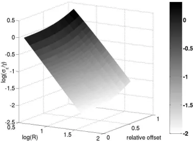
Figure 1 presents the ratio of the standard deviation ofǫXX to the standard deviation of the
Fig. 1.Standard deviation onǫXXas a function of the spanRand the offset, logscale
The reconstruction operatorMcan actually be split in two parts, one dimensionless part that de-pends on the spatial distribution of the data points (mainly their number) and one part introducing the physical size of the neighbourhood, related toR. It writes as follows:
M=D−R1Madi =⇒ cov({δa})=σb2D−R1MadiMTadi | {z }
A D−1
R (5)
whereMadiandAtake the position and number of points of the neighbourhood into account.Ddeals
with the physical size of the neighbourhood, related toR.
The variances on the displacement and its first derivative are hence given by:
– displacement - order 0 field : cov(a1)=A11
– strain - order 1 field : cov(a2)= 1 R2A22
(6)
The terms of the matrixAtend to 0 almost as the inverse of the number of points implied in the reconstruction. In a practical case, as the radiusRincreases, both the physical size of the neighbour-hood and the number of points increase,AandDare hence both modified and tend to 0. One can note that the filtering rate with respect toRon the derivative is larger than on the displacement itself (but its initial value is also larger).
3 Space-Time Diffuse Approximation filtering
In the case where a large amount of images are available for a given test, it is possible to improve the spatial resolution of the reconstructed strain by filtering on space and time at once. The measured displacement fields are therefore stacked together along time, so that we now seek a diffuse field of a three-dimensionnal variableX=(x,t). The approximated field is written as follow:
uap(X)=p(X)Ta(X) with, X=(x,t) (7)
The weighting function defining the neighbourhoods are simply extended to the space-time frame-work:
w(X,Xi)=wre f(x−xi Rx )wre f(
y−yi Ry
)wre f(t−ti
Rt ) (8)
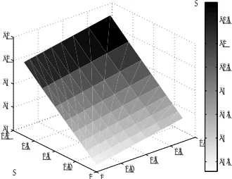
on the filtering of the noise on the measurements can be studied from a theoretical point of view, as presented in Section 2.3 for the 2D diffuse approximation. The relative variance onǫXX is presented
on Figure 2. One can note that the filtering rate related toRton the first derivative is lower than the
one related toRx. This can be explained from the remark from equations (6), noting that an increase
of the span in the direction of the estimated gradient yields a better filtering than in other directions.
0.2 0.4 0.6 0.8 1 0.2 0.4 0.6 0.8 1 −5 −4 −3 −2 −1 −4.5 −4 −3.5 −3 −2.5 −2 −1.5
Fig. 2.Relative random error for Space-time Diffuse Approximation
4 Application to a tensile test on an interlock composite
4.1 Detection of local non-linearities - Spatial Diffuse Approximation
In this section, theǫXXstrain field is studied along a traction test on an interlock composite [8] in order
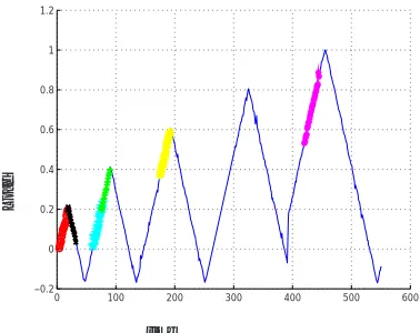
to detect the development of local-nonlinearities. The following example is based on a±45◦traction test on an interlock carbon composite with several loadings and unloadings as described in Figure 3. Digital Image Correlation (DIC) is performed on about 500 images coming from the test, a large number of pictures is thus available. The DIC is performed with CorreliQ4 [9], with aZOIof 8pixels. From the ideas proposed in [10], one can define the linear approximation of the strain at each pixel on several parts of the test. As represented on Figure 3, six different parts of the test are chosen for this study, each made up of about 20 snapshots. For each part, the linear response is estimated from the correspondingNksnapshots,i∈ {1, ..Nk},Fibeing the corresponding load , as the slope of the response
of each pixel:
min ǫlink
Nk X
i
Fiǫlink −ǫ(x,Fi) 2
with, for thekthpart (9)
ǫklinrepresents the linear approximation field for a load of 1N.
These fields are represented on Figure 4 for a spanRof 64pixelsfor the different studied parts of the test. Considering Figure 4(a), the mean of the linear approximation on the first three parts is ploted, and will be considered as the elastic strain fieldǫlinre f of the specimen, before damage occurs. The other
maps are refered by their chronological numbers from Figure 3.
From these fields, it is possible to define a gap to the elastic strain for each part as the discrepancy between the linear approximation related to the part and the reference elastic strain field.
∆ǫlink,re f(x)=ǫlink (x)−ǫre flin(x) (10)
These ∆ǫlink,re f fields are drawn on Figure 5 for a span Rof 64pixels. Figure 5(a) gives an idea of
0 100 200 300 400 500 600 −0.2
0 0.2 0.4 0.6 0.8 1 1.2
time
L
oa
d
Fig. 3.Loading as a function of the time - the six studied parts
(a)ǫlinre f (b) part 4 (c) part 5 (d) part 6
Fig. 4.Linear approximation of the strain fieldǫXXfor the various parts
little mechanical discrepancy. Its magnitude is lower than on the following maps. One can note that the strain increases (due to local damage) on the upper part of the zone in a first time, inducing an unloading of the central zone. In a second time, it seems, the damage propagates to the whole zone following alternative±45◦strips damaging and unloading. This tendencie is confirmed by the Figure
(a)∆ǫlin3,re f (b) ∆ǫ4lin,re f (c)∆ǫlin5,re f (d)∆ǫlin6,re f
Fig. 5.Discrepancy to the elastic strain:∆ǫlink,re f (10)
6 where the incremental discrepancy is ploted. This discrepancy is defined as:
(a)∆ǫ4lin,3 (b) ∆ǫlin5,4 (c)∆ǫlin6,5
Fig. 6.Incremental discrepancy field:∆ǫklin+1,k(11)
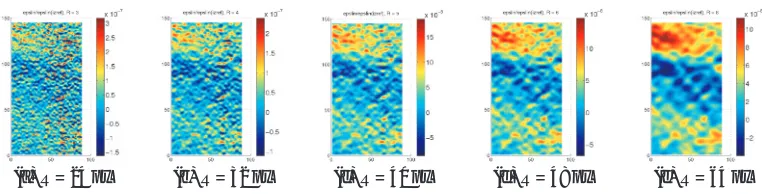
Finally, Figure 7 presents the effect of the spanRon the discrepancy field∆ǫ5lin,re fbetween the strain
coming from part 5 and the reference. On this example, it is obvious that a spanRof 64pixelsis too large and some local information is lost. Thanks to the large number of snapshots (about 60) used for the estimate ofǫlinre f, a good filtering of the noise is achieved and one can afford to take a smaller span Rto get more detailed local nonlinearities. Nonetheless, Figure 8 shows the same reconstruction with same the color range from the linear strain coming from part 3 alone. It can be seen that small spans leads to strains dominated by the noise. A spanRof 64pixels, if too large, allows at least to find out where the main zones of damage appears, in such an example.
(a)R=24px (b) R=32px (c)R=40px (d) R=48px (e)R=64px
Fig. 7.Discrepancy between part 5 and the reference:∆ǫlin5,re f- effect of the spanR
(a)R=24px (b) R=32px (c)R=40px (d) R=48px (e)R=64px
Fig. 8.Discrepancy between part 5 and part 3:∆ǫlin5,3- effect of the spanR
4.2 Comparing spatial Diffuse Approximation and Space-time Diffuse Approximation
From the test described in the previous section, one keeps only the snapshots corresponding to the monotonic loading (leaving the loading-unloading cycles from Figure 3), yielding about one hundred snapshots. One aims at reconstructing the strain field through Space-time Diffuse Approximation. In order to compare the strain field reconstructed here with the linear approximation reconstructed in the previous section, the strain field is divided by the magnitude of the corresponding load.
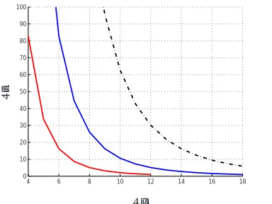
4 6 8 10 12 14 16 18
0 10 20 30 40 50 60 70 80 90 100
Rx Rt
Fig. 9.Isofiltering curves of the Space-time Diffuse Approximation in the (Rx,Rt) plan
From the theoretical filtering presented in Section 3, it is possible to introduce isofiltering curves in the (Rx,Rt) enabling the same filtering of the noise. For a given level of filtering, one can now tune the
time span parameter in order to improve the spatial resolution of the filtering. Sich isofoltering curves are represented Figure 9. One can note that, due to the different behaviour of the spans with respect to the filtering, a given filtering level for a fixed spatial span could lead to a too large time span.
(a)Rx=96px,Rt=0 (b) Rx=48px,Rt=16
Fig. 10.Two isofiltering reconstructions ofǫXX
Figure 10 shows the reconstructed strain (divided by the load level) corresponding to a time in the 6thgroup of Figure 3 (it can therefore be compared to the linear approximation of Figure 4(d)). It is
Diffuse Approximation. Furthermore, when comparing the strain field with the linear approximation of Figure 4(d), it seems the Space-time Diffuse Approximation yields a better spatial resolution.
5 Conclusion
In this paper, the question of the strain reconstruction from full-field displacement measurements has been adressed. A filtering tool based on the the Diffuse Approximation has been proposed, first treating each snapshot apart. Then, an alternative approach based on a coupled space-time filtering has been proposed in order to take advantage of the great amount of snapshots available on some tests. The effect of the spatial and time spans on the filtering has been studied from a theoretical point of view. The filtering approaches have been successfully applied to the detection of early damage on a tensile test on an interlock composite. The example confirmed the ability of the Space-time Diffuse Approximation to improve the spatial resolution.
References
1. A. Kobayashi,Handbook on Experimental Mechanics(Wiley, 1993)
2. M. Geers, R. De Borst, and W. Brekelmans, International Journal of Solids and Structures33-29, (1996) 4293–4207
3. S. Avril, P. Feissel, F. Pierron, P. Villon. Comparison of two approaches for differentiating full-field data in solid mechanics.Measurement Science and Technology, IOP, 21.1,015703 2010.
4. Z. Feng and R.E. Rowlands, Computers and Structures6, (1991) 631-639
5. B. Nayroles, G. Touzot, P. Villon. La m´ethode des ´el´ements diffus.Comptes rendus de l’Acad´emie des Sciences, s´erie 2, M´ecanique, Physique, Chimie, Sciences de l’Univers, Sciences de la Terre, 313-2, 133–138, 1991.
6. W.S. Cleveland, C. LoaderSmoothing by local regression: principles and methods, Springer, 1995. 7. S. Avril, P. Feissel, F. Pierron, P. Villon. Estimation of strain field from full-field displacement noisy
data.Revue Europ´eenne de M´ecanique Num´erique, Lavoisier, 17.5–7,857–868 2008.
8. P. Feissel, J. Schneider and Z. Aboura Estimation of the strain field from full-field displacement noisy data: filtering through Diffuse Approximation and application to interlock graphite/epoxy com-posite, 17thInt. Conference on Composite Materials, 27–31 July 2009, Edinburgh (UK), IOM
9. G. Besnard, F. Hild, S. Roux. Finite-element displacement fields analysis from digital images: Application to Portevin-Le Chˆatelier bands.Experimental Techniques, 46, 789–803, 2006.
10. F Pierron, B. Green and M R Wisnom. Full-field assessment of the damage process of laminated composite open-hole tensile specimens. Part II: Experimental results