Electronic Thesis and Dissertation Repository
2-14-2012 12:00 AM
Confidence Intervals for Comparison of the Squared Multiple
Confidence Intervals for Comparison of the Squared Multiple
Correlation Coefficients of Non-nested Models
Correlation Coefficients of Non-nested Models
Li Tan Jr.
The University of Western Ontario
Supervisor Dr. G.Y. Zou
The University of Western Ontario Joint Supervisor Dr. John Koval
The University of Western Ontario Graduate Program in Biostatistics
A thesis submitted in partial fulfillment of the requirements for the degree in Master of Science © Li Tan Jr. 2012
Follow this and additional works at: https://ir.lib.uwo.ca/etd
Part of the Biostatistics Commons
Recommended Citation Recommended Citation
Tan, Li Jr., "Confidence Intervals for Comparison of the Squared Multiple Correlation Coefficients of Non-nested Models" (2012). Electronic Thesis and Dissertation Repository. 384.
https://ir.lib.uwo.ca/etd/384
This Dissertation/Thesis is brought to you for free and open access by Scholarship@Western. It has been accepted for inclusion in Electronic Thesis and Dissertation Repository by an authorized administrator of
(Spine Title: CIs for Comparison of the Squared Multiple Correlations of Non-nested
Models)
(Thesis Format: Monograph)
by
Li Tan, MSc.
Graduate Program in Epidemiology & Biostatistics
Submitted in partial fulfillment
of the requirements for the degree of
Master of Science
School of Graduate and Postdoctoral Studies
The University of Western Ontario
London, Ontario
February 2012
c
C
ERTIFICATE OF
E
XAMINATION
Joint Supervisor Examiners
Dr. Guangyong Zou Dr. Allan Donner
Joint Supervisor
Dr. Yun-Hee Choi
Dr. John J. Koval Dr. Serge B. Provost
The thesis by
Li Tan
entitled
Confidence Intervals for Comparison of the Squared Multiple Correlation
Coefficients of Non-nested Models
is accepted in partial fulfillment of the
requirements for the degree of
Master of Science
Date
Multiple linear regression analysis is used widely to evaluate how an outcome or
re-sponse variable is related to a set of predictors. Once a final model is specified, the
inter-pretation of predictors can be achieved by assessing the relative importance of predictors.
A common approach to predictor importance is to compare the increase in squared
multiple correlation for a given model when one predictor is added to the increase when
another predictor is added to the same model.
This thesis proposes asymmetric confidence-intervals for a difference between two
cor-related squared multiple correlation coefficients of non-nested models. These new
proce-dures are developed by recovering variance estimates needed for the difference from
asym-metric confidence limits for single squared multiple correlation coefficients. Simulation
results show that the new procedure based on confidence limits obtained from the
two-moment scaled central F approximation performs much better than the traditional Wald
approach. Two examples are used to illustrate the methodology. The application of the
procedure in dominance analysis and commonality analysis is discussed.
KEYWORDS: Coefficient of determination; Multiple correlation coefficient;
Domi-nance analysis; Commonality analysis.
I thank my two advisors Professor Guangyong Zou and Professor John Koval for their
continuous guidance, encouragement and advice throughout my graduate studies and the
number of hours they spent with me on this research. It has been a privilege and a pleasure
to work with mentors with such wisdom and graciousness.
I thank all the friends that I have met over my many years at the University of Western
Ontario. I thank all of the Department of Epidemiology & Biostatistics faculty and staff
members.
Finally, my very special thanks to my farther, mother and brother for their love and
sup-port while I decided to begin another master’s degree for awhile. This thesis is dedicated to
my husband, Jun, who always has confidence in me and whose encouragement is essential
for the completion of my thesis, and also my lovely son, Albert.
Certificate of Examination ii
Abstract iii
Acknowledgments iv
List of Tables vii
List of Figures viii
Chapter 1 INTRODUCTION 1
1.1 Inferences for a single squared multiple correlation . . . 1
1.1.1 Fixed and random regressors . . . 3
1.1.2 Point estimation for a single squared multiple correlation . . . 4
1.1.3 Confidence interval estimation for a single squared multiple corre-lation . . . 6
1.2 Inferences for a difference between two squared multiple correlations . . . 8
1.3 Objective of the thesis. . . 11
1.4 Organization of the thesis . . . 12
Chapter 2 LITERATURE REVIEW 13 2.1 Introduction . . . 13
2.2 Predictor importance in multiple linear regressions . . . 13
2.2.1 Dominant analysis . . . 14
2.2.2 Commonality analysis . . . 15
2.3 Inference procedures for a singleρ2 . . . 16
2.3.1 Point estimator of a singleρ2 . . . 16
2.3.2 Confidence interval construction for a singleρ2 . . . 22
2.3.2.1 Wald-type method . . . 22
2.3.2.2 Fisher’sR2-to-ztransformation . . . 23
2.3.2.3 Exact method . . . 24
2.3.2.4 Approximation methods based on the density ofR2 . . . 24
2.3.2.4.1 A scaled centralF approximation. . . 25
2.3.2.4.2 A scaled noncentralF approximation. . . 28
2.3.2.4.3 A relocated and rescaled centralFapproximation 29 2.3.2.5 Bootstrap method . . . 30
2.4.3 Case 3: Differences between twoρ2s from non-nested models . . . 36
2.5 Summary . . . 36
Chapter 3 CONFIDENCE INTERVAL FOR A DIFFERENCE BETWEEN TWO SQUARED MULTIPLE CORRELATION COEFFICIENTS FROM NON-NESTED MODELS 38 3.1 Introduction . . . 38
3.2 The MOVER . . . 38
3.3 Application of MOVER to differences between two ρ2s from non-nested models. . . 44
3.4 Summary . . . 50
Chapter 4 SIMULATION STUDY 51 4.1 Introduction . . . 51
4.2 Study design. . . 52
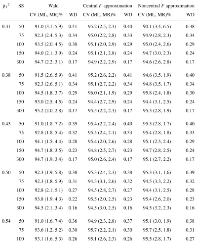
4.3 Results. . . 56
4.3.1 Results for Point Estimation . . . 56
4.3.2 Confidence intervals for a singleρ2 . . . 56
4.3.3 Differences between twoρ2s from non-nested models . . . 57
4.4 Discussion. . . 60
Chapter 5 WORKED EXAMPLES 76 5.1 Introductory remark . . . 76
5.2 Breakfast cereals . . . 77
5.3 Plasma concentrations of beta-carotene. . . 79
5.4 Summary . . . 81
Chapter 6 SUMMARY AND DISCUSSION 89
Bibliography 91
Vita 98
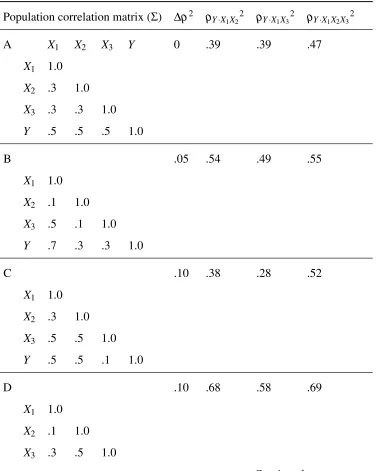
4.1 Population correlation matrices used in simulation studies and the resulting population squared multiple correlation coefficients . . . 61
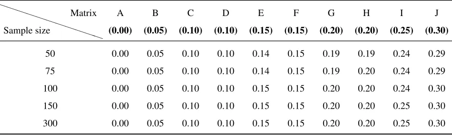
4.2 Sample estimates of the difference∆ρ2averaged over 1000 replications by
sample size . . . 64
4.3 Performance of procedures for constructing two-sided 95% confidence in-tervals for a single squared multiple correlation coefficient over 1000 repli-cations, by sample size. . . 65
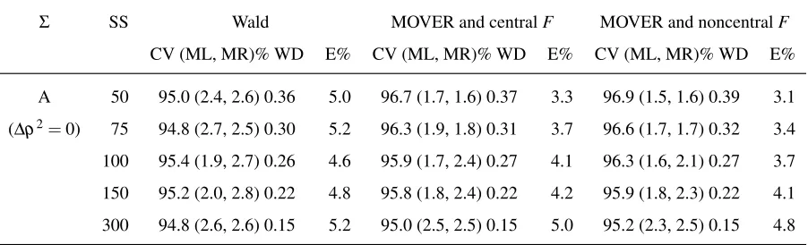
4.4 Null case: the performance of procedures for constructing two-sided 95% confidence intervals for a difference between two ρ2s from non-nested
models over 1000 replications, by sample size.. . . 67
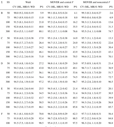
4.5 Non-null cases: the performance of procedures for constructing two-sided 95% confidence intervals for a difference between twoρ2s from non-nested
models over 1000 replications, by population correlation matrix and sample size. . . 68
5.1 Dominance analysis for three predictors . . . 82
5.2 Sample correlation matrix in example of breakfast cereals . . . 83
5.3 Squared multiple correlation coefficients and their asymptotic 95% confi-dence intervals in example of breakfast cereal . . . 84
5.4 Asymptotic 95% confidence intervals for all pairwise differences ofρ2s in
example of breakfast cereal . . . 85
5.5 Sample correlation matrix for variables in example of plasma beta-carotene levels . . . 86
5.6 Squared multiple correlation coefficients and their asymptotic 95% confi-dence intervals in example of plasma beta-carotene levels . . . 87
5.7 Asymptotic 95% confidence intervals for all pairwise differences ofρ2s in
example of plasma beta-carotene levels . . . 88
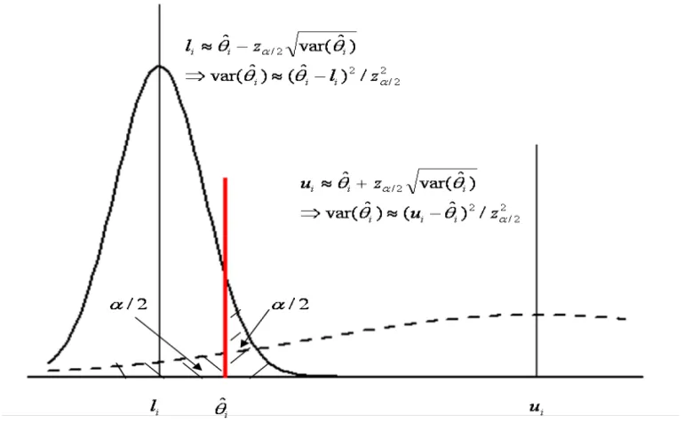
3.1 Confidence limitslianduiforθi . . . 41 3.2 Geometric illustration of margins of errors as obtained using the MOVER . 42
4.1 Coverage rates of 95% confidence intervals over 1000 replications using the Wald-type procedure, by sample size. . . 70
4.2 Coverage rates of 95% confidence intervals over 1000 replications based on a scaled centralF approximation and the MOVER, by sample size. . . . 71
4.3 Coverage rates of 95% confidence intervals over 1000 replications based on a scaled noncentralF approximation and the MOVER, by sample size. . 72
4.4 Power (null hypothesis rejection) rates over 1000 replications using the Wald-type procedure, by sample size. . . 73
4.5 Power (null hypothesis rejection) rates over 1000 replications based on a scaled centralF approximation and the MOVER, by sample size. . . 74
4.6 Power (null hypothesis rejection) rates over 1000 replications based on a scaled noncentralF approximation and the MOVER, by sample size. . . 75
Chapter 1
INTRODUCTION
Multiple linear regression model is one of the most frequently used tools for evaluating
how an outcome or response variable is related to a set of predictors. To quantify the
per-formance of the model, the coefficient of determination is commonly used. All statistical
computer packages provide values of R2 automatically, but without mentioning statistical
inference for its population parameter (ρ2). It is well-known that testing ρ2=0 can be
achieved using anF-test. However, confidence interval construction forρ2 is rarely
men-tioned even though confidence intervals are more informative. The primary goal of this
thesis is to develop inference procedures for quantifying the importance of predictors using
confidence intervals for changes in ρ2. Specifically, we focus on the increase in ρ2 for a
given model when one predictor is added as compared to the increase in ρ2 for the same
model when another predictor is added.
1.1 Inferences for a single squared multiple correlation
The coefficient of determination has several definitions. Generally, R2 is defined as the
proportion of “variability” (measured by the sum of squares) in a data set accounted for
by a multiple regression model (e.g., Steel and Torrie,1960, pg. 187, 287). This interpre-tation is usually presented at the conclusion of a multiple regression analysis. R2 is also
defined as the sample squared correlation coefficient between the response variable and its
corresponding predicted value from the regression model (e.g.,Cohen et al.,2003).
performance of a multiple regression model. A coefficient of determination can represent
a measure of how well the regression line approximates the observed data points. It lies
between 0 and 1. The closer it is to 1, the better is the linear relationship between the
response variable and predictors. The closer it is to 0, the worse is the linear relationship.
The correlation coefficient of 0 indicates no linear relationship between variables, although
nonlinear relationship may exist. However, there also exists some controversy regardingR2
as a goodness of fit statistic (Hagquist and Stenbeck,1998). One argument is that the value ofR2always increases even when a non-predictive regressor is added in a linear regression
model; this can be dealt with by adjusting the R-squared. By including a penalty for the
number of predictors in a model, the adjusted R-squared increases only if the added
predic-tor improves the model more than would be expected by chance (Ezekiel,1930). Another argument is that correlation does not imply causation, since correlation between two
vari-ables may exist due to common causes, confounding varivari-ables or coincidences (Aldrich,
1995). Moreover, even if the causal relationships between the outcome and predictors in two regression models are identical, the value of R2 may differ greatly between different
samples. R2is regarded as more meaningful as a point estimate of populationρ2only for a
data set with random regressors (Helland,1987). For a model with random regressors, the accuracy of R2 depends on not only the sample size, but also the assumed distribution of
predictors.
Besides evaluating the overall performance of a multiple regression model, R-squared
also can be served as a general measure of determining the relative importance of predictors
in multiple regression analysis (Budescu, 1993). After having built a multiple regression model with a chosen set of predictors, one may want to know a relatively important subset
of predictors, or rank the predictors according to their contributions in predicting the
out-come. Hence, it is an important issue in multiple regression analysis to choose an intuitive
and meaningful index of importance for any predictor. There were three classes of measures
of importance including slope-based measures such as regression coefficients, standardized
regression coefficient, correlational measures such as the correlation, the squared
corre-lation and the squared partial correcorre-lation (The coefficient of partial correcorre-lation is defined
as the correlation coefficient between two sets of variables keeping a third set of variable
constant.), and measures based on a combination of the regression coefficients and the
cor-relations such as the product of the correlation between a predictor and the outcome and the
corresponding standard regression coefficient (Azen and Budescu,2003; Budescu, 1993). However, all these measures do not offer an intuitive and universal interpretation of
im-portance which leads to different orderings of the predictors’ imim-portance and confusion on
the meaning of importance. Budescu(1993) suggested that an appropriately general mea-sure of importance should satisfy the following three conditions: “(a) Importance should
be defined in terms of a variable’s ‘reduction of error’ in predicting the outcome; (b) The
method should allow for direct comparison of relative importance instead of relying on
inferred measures; (c) Importance should reflect a variable’s direct effect, total effect and
partial effect.” According to these criteria, Budescu(1993) developed a new methodology – dominance analysis, in which a predictor is considered to be dominant or more important
than another predictor if its additional contribution in the prediction of the response
vari-able defined as the squared semipartial correlation (i.e., the difference between two squared
multiple correlations from nested models), is greater than the competitor’s for all possible
subset models. In a word, one can identify the relative importance of predictors through a
series of pairwise comparisons of squared multiple correlations from all submodels.
1.1.1 Fixed and random regressors
Depending on whether regressors are fixed or random, inference procedures forρ2are
dif-ferent. A key distinction with respect toρ2between fixed-score and random-score multiple
regression models is thatρ2is constant for fixed-score regression models, while population
ρ2can be made arbitrarily small and large when regressors are random.
For a multiple regression model having pfixed predictors and sample size n,
partic-ular, when testing for the null hypothesis H0 :ρ2 =0, one usually construct a statistic
R2/p
(1−R2)/(n−p−1). Under H0, the statistic follows a central F distribution with degrees of
freedom pandn−p−1. Whenρ6=0, the statistic follows a noncentralFdistribution with
degrees of freedom pandn−p−1 and a noncentrality parameter.
In this study, attention is restricted to inference procedures for models with random
regressors. Since inference forρ2arising from fixed regressors can be easily done on the
basis of the noncentralF distribution with degrees of freedom independent ofρ2. For
ran-dom regressors, the same centralF-distributed statistic can be used for testing significance,
because when the null hypothesis is true, the sampling distribution forR2does not change
for fixed or random regressors (Smithson,2003). However, this is not a case if we are inter-ested in confidence intervals for ρ2 in models with random regressors. Since for nonzero
cases, the noncentrality parameter is a function of regressors, the unconditional
distribu-tion of R2 highly depends on the assumed distributions of those regressors. Hence, when
constructing confidence intervals forρ2, many statistical inference procedures suitable for
fixed regressors only can provide conditional confidence intervals on particular values of
random regressors observed in the sample. In fact, since the random regressors themselves
take account of sampling error, the confidence intervals forρ2from fixed regressors models
are much narrower than those from random regressors models (Smithson,2003). Hence, a unconditional confidence interval-based inference forρ2in models with random regressors
is preferred.
1.1.2 Point estimation for a single squared multiple correlation
It is well known that R2 is defined as the ratio of regression sum of squares and the total
sum of squares. According to this definition, one can calculate the value of R2 from the
fitted model. Almost all statistical softwares automatically provide the value of R-squared
for a multiple regression model.
Under the assumption that the joint distribution of the outcome and predictors is
(Hagquist and Stenbeck, 1998). However, R2 usually has a positive bias as an estimate of ρ2, especially when the number of regressors are moderate or large. Many researchers
have developed various alternatives that reduce the bias (see Raju et al., 1997). A com-monly used estimator is the R2 adjusted by replacing the sum of squares with the mean
square by (Ezekiel, 1930). Alf and Graf(2002) comparedR2 and eight other estimates of
ρ2, which includes Smith’s estimator (Ezekiel, 1929), an estimator proposed by Wherry
(1931), the adjustedR2 (Ezekiel, 1930), a unbiased estimator (Olkin and Pratt,1958) and its two approximate versions proposed by Pratt and presented in Claudy (1978) and by
Herzberg (1969), a empirically based estimate (Claudy, 1978), and the maximum likeli-hood estimate (Alf and Graf,2002). The first two have similar modifications to the adjusted R2by including a penalty for the number of predictors in a model, and the other five
estima-tors involving the unbiased estimate provided by Olkin and Pratt (1958) are derived from models with random regressors. Alf and Graf(2002) found that: ‘the adjustedR2(Ezekiel,
1930) was unbiased only whenρ2is 0’;Olkin and Pratt(1958)’s estimator is unbiased over
all the values of the sample size n and ρ2, but involves a complex hypergeometric
func-tion; and the remaining estimators (includingR2and a maximum likelihood estimate ofρ2
derived from its exact density function) were biased for all the values ofnandρ2.
Another way to compute theR2of a regression model requires the sample simple
cor-relations among the dependent variable and predictors within the model. According to the
definition (Pearson and Filon,1898), a multiple correlation coefficient can be mathemati-cally represented as a function of simple and/or partial correlation coefficients, while partial
correlations are also functions of simple correlations. Correspondingly, as a sample squared
multiple correlation coefficient,R2 can be represented as a function of sample simple
cor-relation coefficients. This cor-relationship also can be represented in matrix form. That is, R2
can be represented as a function of several determinants of matrices of the sample simple
correlations between variables included in the model (Olkin and Siotani,1976). These for-mulas based on correlation matrices are easily used to estimate ρ2 of a regression model
1.1.3 Confidence interval estimation for a single squared multiple correlation
Several confidence interval procedures for a single ρ2 in random scores models have
ap-peared in the literature. These procedures include a Wald-type confidence interval, a
confi-dence interval based on Fisher’sR2-to-ztransformation, a confidence interval derived from
the exact density of R2, asymptotic confidence intervals based on various approximations
to the density of R2, and bootstrap confidence intervals which do not assume multivariate
normality for the outcome and regressors.
With an estimator of the asymptotic variance of R2 provided by Wishart (1931), the Wald method can be used to construct a symmetric confidence interval of ρ2. However,
the forced symmetry of the Wald-type confidence interval is questionable, since the
sam-pling distribution of R2is skewed and converges very slowly to normality (Algina,1999). Furthermore, this Wald-type confidence interval constructed by using ordinary R2 and its
variance estimate may be out of range of 0 to 1. Meanwhile, if one uses the adjustedR2and
its variance estimate instead of ordinaryR2and its variance estimate, since the adjustedR2
has a much bigger variance estimate thanR2does, the resulting lower Wald-type confidence
limit forρ2may be negative, which is inconsistent with that of the associatedFtest.
Fisher’sztransformation which is commonly used for inferences on simple correlations
has been applied to make inferences on squared multiple correlations. The confidence limits
forρ2can be represented as a monotone increasing function of confidence limits of Fisher’s
z statistic, which is assumed to be approximately normally distributed. However, Fisher’s
statistic, since it takes only non-negative values, has a more positive skewed distribution
than R2 (Algina, 1999). Therefore, it is not recommended that Fisher’s transformation is used for constructing confidence intervals forρ2.
Under the multivariate normality assumption, Fisher(1928) derived the exact density function of R2. Due to the complex form of the density, it is impossible to derive an
an-alytical confidence interval for ρ2 from the density, although lower confidence limits for
Lee, 1972). Various asymptotic confidence intervals for ρ2 have been proposed through
approximating a transformed variableR2/(1−R2)to be scaled centralF distributed ( Gur-land,1968;Helland, 1987), scaled noncentralF distributed (Lee,1971), and relocated and rescaled centralFdistributed (Lee,1971). The comparison between the exact and three ap-proximate density functions of R-square shows that the scaled noncentralF approximation
which requires the estimation of the noncentrality parameter performs much better than that
of the relocated and rescaled centralF approximation, while slightly better than that of the
scaled centralF approximation.
Bootstrap methods first proposed byEfron(1979) may be thought to provide a univer-sal solution to inference, especially for those estimators having an unknown or complicated
distribution. The bootstrap aims to use computer-based re-sampling to approximate the
sampling distribution of the estimate of the parameter. Common bootstrap methods for
constructing confidence intervals are the percentile (Schenker, 1985), the bias-corrected (BC) (Efron, 1981), the bias-corrected and accelerated (BCa) (Efron, 1987), bootstrap-t (Efron, 1979), and the approximate bootstrap confidence intervals (ABC) (Efron and Tib-shirani, 1993). However, there are limitations to these bootstrap methods (Efron, 1987;
Efron and Tibshirani, 1993). For example, the percentile interval performs well only for unbiased statistics having a symmetric sampling distribution; the BC method requires the
existence of a normalizing transformation and stabilized variance, and is applicable only
for large samples; the validity of the BCa method highly depends on the accuracy of
esti-mating an extra acceleration constant; the bootstrap-tmethod requires an accurate estimate
of the standard error of the statistic and often yields a very wide confidence interval; the
ABC is applicable for smoothly defined parameters in exponential families and also
re-quires an estimate of the nonlinearity parameter. Furthermore, nonparametric methods like
jackknifing and bootstrapping are more sensitive to the sample size than valid parametric
methods. A cautionary example shows that all jackknife and bootstrap confidence intervals
ofρ2perform too poorly to be trusted for a data set with small sample size and relatively
inter-vals require intensive computations, hence, asEfron(1988) stated, the bootstrap can be an alternative method only when there is no any suitable parametric methods.
In summary, the scaled centralF approximation (Gurland, 1968;Helland, 1987) and the scaled noncentralF approximation (Lee, 1971) may be good choices to construct fidence interval for a single squared multiple correlation coefficient. Furthermore, the
con-fidence intervals based on these two approximations are easily obtained by respectively
implementing existing statistical package programs, such as SAS PROC CANCORR, a
SAS macro or an SPSS syntax provided by (Zou,2007).
1.2 Inferences for a difference between two squared multiple correlations
As mentioned before, a squared multiple correlation is an important measure for
quantify-ing the overall performance of a model, and also for quantifyquantify-ing the importance of a set
of predictors. Explicitly, comparisons ofR2s from all possible linear regression submodels
involving various sets of predictor, are made to identify a relatively important subset of
predictors, or rank the predictors according to their contributions in predicting the response
variable. Both are the final objectives of two popular research fields (Azen and Budescu,
2003; Hedges and Olkin, 1981), dominance analysis (Budescu, 1993) and commonality analysis (Kerlinger and Pedhazur,1973).
The exact sampling distribution of a singleR2 is already highly complex, so we may
have to resort to the joint asymptotic distribution theory of two or more squared multiple
correlations. For models with random regressors, the joint distribution of simple
correla-tions or funccorrela-tions of correlacorrela-tions (e.g., squared multiple correlation) among the response
variable and regressors highly depends on the distribution of the depended variable and
independents.
When the outcome and regressors are assumed to be multivariate normal, most
litera-tures have presented the asymptotic joint distributions of functions of correlations including
de-terminants of correlation matrices (Olkin and Siotani,1976), squared multiple correlations (Hedges and Olkin, 1981), any sets of partial and/or multiple correlations (Hedges and Olkin, 1983), and so on. Each of these joint distributions is asymptotically multivariate normal by applying the central limit theorem. However, these asymptotic joint
distribu-tions are only applicable for very large samples, since the exact joint distribution of two
correlatedR2s is probably still extremely skewed.
Without the multivariate normality assumption for a vector variate of interest, Steiger and Hakstian(1982) presented an asymptotic joint distribution of simple correlations among variables involving the kurtosis of a vector of variables. In particular, when the joint
distri-bution of variables belongs to elliptical family, the asymptotic variance-covariance matrix
of correlations can be obtained through multiplying the asymptotic variance-covariance
matrix derived under the multivariate normality assumption (Olkin and Siotani,1976) by a relative kurtosis. This relative kurtosis is equal to 1 when the variables have a multivariate
normal distribution. The coefficient of multivariate kurtosis can be estimated by using the
algorithm provided byMardia and Zemroch(1975). According to this asymptotic theory,
Steiger and Browne(1984) presented a series of chi-square tests for linear combinations of partial correlations, independent or correlated multiple correlations, and canonical
correla-tions, with or without the assumption of multivariate normality. However, this asymptotic
theory is complicated except for particular cases, for example, elliptical families.
It has been known that confidence intervals can provide us a quantitative measure of an
effect, not just a qualitative impression, that is, whether the effect is statistically significant.
Hence, we are interested in not only whether the differences between two squared multiple
correlations is positive or negative, but also the confidence intervals for the difference.
The relationships between any two regression models can be classified into three
cate-gories: independent, nested (i.e., all predictors within a model are a part of the predictors
of another model), and overlapped but non-nested (i.e., two models have a common subset
of predictors). Hence, inferences for differences between two R2s should be made in the
A comparison of R2s from two models without any common predictors or from two
independent populations is the simplest case due to the independence between two R2s.
Based on inference procedures for a singleR2, one can easily extend to inferences for
dif-ferences between two independent population ρ2s. Because a single R2 has a positively
skewed density, the distribution of a difference between two independent R2s is probably
still skewed. Hence, the Wald-type interval estimation for the difference of two
indepen-dent R2s presented in Olkin and Finn (1995) still has its inherent deficiency (see Algina,
1999), which forces a confidence interval to be symmetric for those parameters whose sample estimates having skewed distributions. Later, Chan (2009) described a bootstrap confidence interval about a difference between two independent R2s which involves
inten-sive computations. Zou(2007) proposed simple and direct confidence interval construction for a difference between two independentR2s by using a recovered variance estimate from
confidence limits for each R2. The rationale behind this method is termed the Method of
Variance Estimates Recovery (MOVER) (Zou,2008). Given confidence limits for each of two parameters and their correlation coefficient, as a general approach, the MOVER can be
used to construct confidence intervals for the difference, the sum or the ratio of those two
parameters. This approach takes into account the skewness of some sampling distributions,
so that the MOVER performs well for a wide range of parameters in terms of both coverage
rate and interval width, even for small to moderate sample sizes.
Other two cases including the comparisons of twoR2s from nested or non-nested
mod-els need to consider the correlation between two R2s. Olkin and Siotani (1976) derived asymptotic covariance estimates between any two simple correlation coefficients. Using
these asymptotic covariance estimates,Olkin and Finn (1995) suggested a Wald-type con-fidence interval for differences between two correlated squared multiple correlations or a
squared partial and a squared multiple correlation. Consider the difference between two
squared multiple correlations: first, any difference between twoR2s can be represented as
a function of sample simple correlation coefficients, since a multiple correlation can be
for the sample simple correlation coefficients involved in the function, one can obtain the
asymptotic variance estimate of the difference by using the delta method; finally, according
to the central limit theorem, one can construct a Wald-type confidence interval for this
dif-ference between two correlatedR2s.Graf and Alf(1999) improvedOlkin and Finn(1995)’s approaches for further simplification. Through a simulation study, Azen and Sass (2008) examined the performance of the Wald-type confidence interval for differences between
two R2s from non-nested models proposed byOlkin and Finn (1995) and found that this asymptotic confidence interval is acceptable in terms of coverage rate only for large sample
size (>200).
1.3 Objective of the thesis
The poor performance of existing confidence interval procedures for differences between
two correlated squared multiple correlation coefficients may lead us to wrong conclusions
on the relative importance of predictors. The main reason is that the existing Wald-type
confidence interval constructions proposed by Olkin and Finn(1995) ignore the potential skewness of the sampling distribution for a comparison ofR2s. Furthermore, this procedure
based on the central limit theorem has been shown to be accepted only for large samples
(>200).
The objective of this study is to provide a simple and efficient inference procedure for
differences between two correlated R2s from non-nested models. In particular, under the
multivariate normality assumption, we propose a closed-form confidence interval for the
comparison of the changes in R2 when each of two predictors is added to a model with
some essential predictors.
Inspired by the good performance of the MOVER proposed byZou(2008) applied in constructing a confidence interval about a difference between two independent ρ2 (Zou,
confidence intervals to be symmetric and also not require the normality assumption of
sam-ple estimate of parameter of interest, and thus may improve the performances of the existing
confidence intervals for differences between two correlatedρ2s from non-nested models.
The performance of the proposed confidence interval will also be evaluated and
com-pared to that of the existing Wald-type confidence interval provided by Olkin and Finn
(1995).
1.4 Organization of the thesis
In this study, Chapter 2 reviews background on determining the relative importance of
pre-dictors, as well as literatures regarding inferences procedures for a single squared multiple
regression and differences between two squared multiple regression. Chapter 3 first
de-scribes the MOVER proposed in the paper of Zou(2008), then presents a new confidence interval construction for differences between two correlated squared multiple correlations
from non-nested models. In Chapter 4, a simulation study compares the performance of our
proposed confidence interval to that of the existing Wald-type confidence interval proposed
Chapter 2
LITERATURE REVIEW
2.1 Introduction
As outlined in Chapter 1, changes in squared multiple correlation may be used to evaluate
the relative importance of predictors in multiple linear regression models. In this chapter,
we first review predictor importance in the context of multiple linear regressions, then
de-scribe some main approaches for constructing confidence intervals for a single R2and for
differences between two independent and correlatedR2s.
2.2 Predictor importance in multiple linear regressions
With data of a sample of a response variable and a large set of potential predictors, we may
build a model using a two-stage process (seeAzen et al., 2001;Budescu, 1993). First, we identify a subset of predictors that can adequately describe the relationship between the
de-pendent variable and predictors. This stage is usually referred to as model selection. Once
a model is selected, we may proceed to interpret the model by comparisons of predictor
importance.
In the model selection stage, there are two general approaches termedexplanation and
prediction (Pedhazur,1982). The explanation approach may also be regarded as the con-ception of causation. Based on previous theory or substantive research, those predictors
which are conceived to be associated with the dependent variable are identified and then
included in the model. The prediction approach aims to find the most predictive model,
re-gardless of the underlying mechanism of how the predictors affect the response. A variety
Informa-tion Criterion (AIC) (Akaike,1974) and the Bayesian Information Criterion (BIC) (Akaike,
1977).
Having built a model with a chosen set of predictors, we may then assess a relatively
important subset of predictors, or rank the predictors according to their contributions in
predicting the response variable. They are the final objective of dominant analysis and
commonality analysis, respectively (Azen and Budescu,2003;Hedges and Olkin,1981).
2.2.1 Dominant analysis
In order to identify the most important set of predictors from ppotential independent
vari-ables, we can compare all 2p−1 regression models with each model involving a subset of p predictors and a dependent variable in terms of certain indices. These indices include
simple correlations, regression weights, partial and semi-partial correlations, and squared
multiple correlations. Among them, the squared multiple correlation R2 for a multiple
re-gression model is shown to preferable (Budescu,1993).
Budescu(1993) proposed dominance analysis as a new approach to evaluate the rela-tive importance of predictors in multiple linear regression. Here, dominance is a pairwise
relationship, indicating that one predictor dominates another if it is more useful than its
competitor in all regressions. Explicitly, given a model with a set of essential predictors,
it is defined that a set of additional potential predictors is more important than the other
sets, if it increases the model’sR2 more than the other sets do. After estimating the
sam-ple squared multisam-ple correlations,R2s, for all 2p−1 regression models, then comparing all these R2s, we can identify the relative important set of predictors. In particular, suppose
that in a model with X1 and X2 as essential predictors, to determine the dominance of X3
andX4, we can compare theR2 increase whenX3 is added to the model to that whenX4is
2.2.2 Commonality analysis
The objective of commonality analysis is to partition the variance of the response variable
accounted for into the unique and combined contributions a predictor makes. It assesses
the individual and collective effects of a set of predictors on a single dependent variable,
such as the individual and collective effects of school and social background on educational
achievement. Its description can be found in many textbooks on regression analysis in the
social sciences, such asKerlinger and Pedhazur(1973).
After the equality of educational opportunity report (Coleman et al., 1966) created the controversy that there was no general methods of assessing the relative importance of
cor-related predictors, many papers dealt with methods of assessing or describing the relative
contribution of correlated predictors. Commonality analysis was first advocated by Mood
(1971) as a tool for developing learning models. It has been used in educational research such as school effect studies (Pedhazur, 1975), teaching studies (Dunkin, 1978). Later,
Newton and Spurrell(1969a,b) developed this technique in industrial sciences and called it “element analysis”.
Commonality analyses can be illustrated as follows. Suppose we are given the squared
multiple correlation of a model with the response variableY and two predictorsX1andX2,
ρY·X1X2
2, then we can partition
ρY·X1X2
2into three parts:
γ1,γ2andγ12. We have
γj= the unique contribution ofXjtoρY·X1X2
2, j=1,2,
γ12 = the common contribution ofX1andX2toρY·X1X2
2,
where the last termγ12 is called the commonality ofX1andX2. The above definitions lead
to the following system of equations:
ρY·X1X2
2 =
γ1+γ2+γ12
ρY X1
2 =
γ1+γ12,
ρY X2
2 =
where ρY X1
2 and ρ
Y X2
2 are squared multiple correlation of a model predicting Y from a
single predictorX1orX2, respectively.
It was suggested that the rule of selecting predictors should be based on large unique
components and small commonalities (Newton and Spurrell,1969a,b;Mood,1971). Hence, from the perspective of commonality analysis, a series of comparisons ofR2s is an
impor-tant tool of determining predictor importance (Hedges and Olkin,1981).
2.3 Inference procedures for a singleρ2
Before presenting procedures for the comparison ofR2s, we describe inference procedures
for a single ρ2. In particular, we start with point estimators of a single population squared
multiple correlationρ2, includingR2and other estimators which are designed to reduce the
potential bias of R2 as an estimator of population parameterρ2. This parameter also can
be estimated in terms of simple and/or partial correlations, which is easily calculated by
using a handy calculator for small number of predictors, given the correlation matrix for
a dependent variable and predictors. We then introduce five procedures for constructing a
confidence interval for ρ2. These procedures include the Wald-type symmetric confidence
interval based on the asymptotic variance, a confidence interval based on the Fisher’s exact
density ofρ2(Fisher,1928), confidence intervals based on various approximated density of ρ2, a bootstrap confidence interval, and a confidence interval developed byGurland(1968)
andHelland(1987).
2.3.1 Point estimator of a singleρ2
Consider a multiple linear regression model
y=1β0+xβ+,
wherey= (y1,y2, . . . ,yn)0, an×1 vector1= (1,1, . . . ,1)0,β0andβ= (β1,β2, . . . ,βp)0are
(When regressors are random, the mean and variance ofare conditional onx), and each
row ofn×pmatrixxis a sample of a vector consisting of ppredictorsX= (X1,X2, . . .Xp),
Let ¯Y and ¯Xrespectively be the sample mean of dependent variableY and the vectorX,
and letex=x−1X, then the least square estimators for¯ β0andβare
b
β0 = Y¯−X¯βb,
b
β = ex0ex−1ex0y,
and the predicted vector is given by
by = 1βb0+xβb.
The population multiple correlation coefficient ρ2 can be defined as the correlation
betweenY and Xβ, sinceXβ is the linear combination of variablesX1,X2, . . .Xp that has maximal correlation withY (Pearson,1912). SinceY =β0+Xβ+ε andε is independent
ofX, according to the definition,ρ2can be written as
ρ2 = [cov(Y,Xβ)] 2
var(Y)var(Xβ)
= var(Xβ)
var(Y) .
When regressors are random, we usually assume thatXhas a multivariate normal
distribu-tion with meanµxand variance-covariance matrixΣx.
ρ2 = β
0
Σxβ
σ2+β0Σxβ
. (2.1)
The total, regression and error sums of squares are respectively presented by
SST =
n
∑
i=1
(yi−Y¯)2= (y−1Y¯)0(y−1Y¯),
SSR =
n
∑
i=1
(ybi−Y¯)2
= (by−1Y¯)0(by−1Y¯) =βb0 e
x0exβb,
and the coefficient of determination is defined by
R2= SSR
SST.
Because
b
σ2= SSE
n−p is a unbiased estimator ofσ2and
Sx=
1 n−1ex
0
ex=
1
n−1(x−1X¯)
0(x−1X¯)
is an unbiased estimator ofΣx, thenR2becomes
R2= (n−1)βb
0S
xβb
(n−p)σb2+ (n−1)βb0Sxβb .
Due to the similarity of this representation and the formula (2.1),Helland(1987) concluded that only for random regressors, can R2 be treated as a estimator of ρ2. This conclusion
is based on the multivariate normality assumption for random regressors, so it is not
suit-able for models with fixed regressors. Although most articles described theR2in computer
programmes as an estimator of populationρ2, Helland(1987) clearly pointed out the
pre-condition of this usage.
R2 has a positive bias as an estimator of population ρ2, especially when the number
of regressors are moderate or large. To correct for the bias inR2, at least eight alternative
estimators have been proposed in the literature.
1. Smith’s estimatorρbS2(Ezekiel,1929) has a form of
b
ρS2 = 1− 1−R2 n
n−p.
b
ρS2shrinks a lot, but it increases as more predictors are added.
2. By replacingσ2andΣxin the formula (2.1) with their respective unbiased estimators
b
σ2andSx,Wherry(1931) definedρb
2
W as
b
However, this replacement does not makeρb
2
W unbiased as an estimator ofρ2; it has
been shown thatρb
2
W overestimatesρ2(Wherry,1931).
3. Ezekiel(1930) proposed adjustingR2by replacing sum of squares with mean squares in ordinaryR2, giving
R2ad j = 1− 1−R2 n−1 n−p−1.
Huberty and Mourad (1980) found thatR2ad j adequately estimated ρ2. Hence,R2ad j is a commonly used alternative of R2, and is provided by most statistical computer
packages.
4. Based on a random regressor model, Olkin and Pratt (1958) provided an unbiased estimator ofρ2as
b
ρOP2 = 1− 1−R2 n−3
n−p−1F
1,1;n−p+1
2 ;(1−R
2)
,
whereF(·)is the hypergeometric function. This estimator can be written in a closed form as
b
ρOP2 = 1− 1−R2 n−3
n−p−1
1+2(1−R
2)
n−p+1 +
8(1−R2)2 (n−p−1)(n−p+3)
.
5. By approximating to the hypergeometric function F, Pratt developed an estimator
ρP2, which is also presented inClaudy(1978) as
b
ρP2 = 1− 1−R2 n−3
n−p−1
1+ 2(1−R
2)
n−p−2.3
.
Claudy(1978) found thatρP2underestimatesρ2.
6. Herzberg(1969) also gave another approximate estimator
b
ρH2 = 1− 1−R2 n−3
n−p−1
1+2(1−R
2)
n−p+1
.
7. Claudy(1978) developed an empirical estimate as
b
ρCL2 = 1− 1−R2 n−4
n−p−1
1+2(1−R
2)
n−p+1
,
whileRaju et al.(1997) found thatρb
2
CL is biased for estimatingρ2.
8. For fixedn, pandR2,Alf and Graf(2002) obtained the maximum likelihood estimate ofρ2,ρb
2
MLE, by maximizing the exact density function ofR2(Fisher,1928).
Alf and Graf(2002) compared R2 and other eight versions of estimates of ρ2. They
found that the estimator provided by Olkin and Pratt (1958) performed well over a wide range of values for nand ρ2; the adjusted estimator for ρ2 (Ezekiel, 1930) was unbiased
only when the population ρ2 was 0, and the remaining estimators includingR2 andρb
2
MLE
were biased for all the values of n and ρ2. The above evaluations are based on the
as-sumption that the joint distribution of independent and dependent variables is multivariate
normal. If the normality assumption is violated, the evaluations become very complex (see
Drasgow and Dorans,1982).
The multiple correlation coefficient can be represented as a function of simple and
par-tial correlation coefficients. Therefore, once we know the correlation matrix for a response
variable and predictors, we can estimate any multiple correlation coefficient.
Let ρY·X1X2...Xp be a population multiple correlation, which measures the strength of
the linear relationship between a dependent variableY and a set of independent variables
X1,X2, . . . ,Xp. In other words, it also can be explained as the maximum correlation coef-ficient between Y and all linear combinations ofX1,X2, . . . ,Xp (Pearson, 1912). Squared multiple correlations can then be mathematically represented as functions of simple and/or
partial correlations (Pearson,1912;Olkin and Siotani,1976). For example, the coefficients of multiple correlation involving the first two or three variables, denoted as ρY·X1X2 and
ρY·X1X2X3 respectively, are given by
1−ρY·X1X2
2 = 1−
ρY X1
2
1−ρY X2·X1
2
(2.2)
1−ρY·X1X2X3
2 = 1−
ρY X1
2
1−ρY X2·X1
2
1−ρY X3·X1X2
whereρY X2·X1 andρY X3·X1X2are two partial correlations. A partial correlation is also referred
to as adjusted correlation. For example,ρY X2·X1is the correlation of variablesY andX2, after
removing the association of each withX1, given by
ρY X2·X1 =
ρY X2−ρY X1ρX2X1
p
(1−ρY X1
2) (1−ρ
X2X1
2) (2.3)
ρY X3·X1X2 is the partial correlation of variablesY and X3 keeping variablesX1andX2
con-stant, then
ρY X3·X1X2 =
ρY X3·X2−ρY X1·X2ρX3X1·X2
p
(1−ρY X1·X22) (1−ρX3X1·X22)
= ρY X3·X1−ρY X2·X1ρX3X2·X1
p
(1−ρY X2·X1
2) (1−ρ
X3X2·X1
2)
Combining equations2.2and2.3, we have
ρY·X1X2
2 =
ρY X1
2+
ρY X2·X1
2
1−ρY X1
2
= ρY X1
2+ ρY X2
2−2
ρY X1ρY X2ρX1X2
1−ρX1X22
The relationships among correlations also can be easily represented in matrix form
(Olkin and Siotani,1976). LetΣ(S) =Σ(s1,s2, . . . ,sm)andbΣ(S) =bΣ(s1,s2, . . . ,sm)
repre-sent the population and sample correlation matrices for variablesXs1,. . .,Xsm, respectively. LetρY·Xα
2be the population squared multiple correlation betweenY and a set of variables
with subscriptsα;ρY X1·Xα
2be the population squared partial correlation betweenY andX 1
for fixed variables with subscripts α; ρY Xα·Xβ
2 be the population squared partial-multiple
correlation betweenY and a set of variables with subscriptsα while keeping a set of
vari-ables with subscriptsβ fixed, then
ρY·Xα
2 = 1−|Σ(0,α)|
|Σ(α)|
ρY X1·Xα
2 = |Σ(0,1,α)|
p
|Σ(0,α)| · |Σ(1,α)|
ρY Xα·Xβ
2 = |Σ(β)| · |Σ(0,α,β)|
where α and β are two sets of subscripts, |Σ(α)| is the determinant of the population
correlation matrix for variables with subscriptsα,|Σ(0,α)|=(ρi j)
is the determinant of
the population correlation matrix for the response variableY and variables with subscripts
α. Similar definitions for other determinants of population correlation matrices.
Note that these formula are also suitable for sample correlations by replacingρ andΣ
with sample correlation coefficientsrand matrixΣb, respectively.
2.3.2 Confidence interval construction for a singleρ2
There are several approaches to constructing confidence interval for a singleρ2. These
ap-proaches can be classified into five categories. Herein, these five categories of apap-proaches
are presented respectively as follows. Among these five approaches, a confidence interval
developed byGurland(1968) andHelland(1987) based on a scaled centralF approxima-tions to the density ofR2/(1−R2)performs well.
2.3.2.1 Wald-type method
The variance ofR2was originally derived byWishart(1931), given as
var(R2) = 4ρ
2 1−
ρ22(n−p−1)2
(n2−1) (n+3) .
Whennis large, the variance can be approximated by
var(R2) ≈ 4 nρ
2 1− ρ22
1−2p+5 n
.
If 2p+5 is small relative ton, the expression reduces further to
var(R2) ≈ 4ρ
2 1−ρ22
n . (2.4)
Hence, 100(1−α)% confidence limits for ρ2 by using the Wald method is given by R2±zα/2pvarc(R2), where
c
var(R2)is the sample estimate of var(R2)withρ2replaced by
From equation (2.4), we can see that whenρ2=0, the variance estimate ofR2is 0, so
that the Wald method cannot be used. The method is more suitable for cases with symmetric
sampling distributions, but not forρ2, since the sampling distribution ofR2 is skewed and
converges very slowly to normality (Algina, 1999). Furthermore, this method may give confidence limits out of range of 0 to 1.
2.3.2.2 Fisher’s R2-to-z transformation
Another method of interval estimation for ρ2 is based on Fisher’sz transformation of R2
rather thanr(seeOlkin and Finn,1995). Fisher’zstatistic
z=log
1+R 1−R
=log 1+ √
R2
1−√R2
!
is approximately normally distributed with meanE(z) =ζ =log[(1+pρ2)/(1−pρ2)]
and variance 4/n(Algina,1999). Then the confidence limits ofz,lz anduz, have forms
log 1+ √
R2
1−√R2 !
±zα/2p4/n.
Sincezis a monotone increasing function ofR2, if bothlz anduz are non-negative then the confidence limits forρ2are given by
exp(lz)−1
exp(lz) +1
2 ,
exp(uz)−1
exp(uz) +1
2
and iflz<0 then the lower confidence limit forρ2is 0.
Note that the confidence interval based on Fisher’s z transformation performs more
poorly than others (Algina, 1999). The main reason is that the limiting distribution of Fisher’s transformation on R2failed to approach normality asymptotically (Gajjar, 1967). AsR2 ranges from 0 to 1, the transformed values of Fisher’szonly covers the range from
0 to plus infinity. Therefore, Alf and Graf (1999) pointed out that, “Fisher’sz values are severely truncated in the lower tail, resulting in a distribution that is even more positively
skewed than is the original distribution of squared multiple correlations” (p. 74). In
2.3.2.3 Exact method
Based on the geometrical interpretation of multiple correlations, Fisher (1928) gave the exact density function ofR2, which is later written in the following form (Lee,1972)
fR2(x) = B(p/2,n1/2)−1 1−ρ2
(n−1)/2
(x)p/2−1(1−x)n1/2−1
F (n−1)/2,(n−1)/2;p/2;ρ2x (2.5)
whereB(.) andF(.)respectively denote the beta and Gaussian hypergeometric functions,
n1=n−p−1,nbeing the sample size.
We know that both beta and Gaussian hypergeometric functions are complicated
in-tegrands or series. There is also no closed formula for calculating the exact cumulative
distribution function of R2. Therefore, the calculation of exact confidence limits requires
iterations on computing the percentiles of the integral of density fR2(x). Based on this
distribution, Kramer(1963) and Lee(1972) tabulated only upper percentage points of the distribution ofρ2and limited to confidence levels 5% and 1% in particular cases. A
stand-alone program, “R2”, available athttp://www.statpower.net , has been developed for
obtaining the confidence limits based on this distribution (Steiger and Fouladi,1992).
2.3.2.4 Approximation methods based on the density of R2
Due to the complexity of the exact density of R2, many researchers developed various
methods of obtaining approximate confidence intervals forρ2, through asymptotically
ex-panding or approximating the density function ofR2. Several asymptotic procedures have
appeared in the literature, including a two-moments scaled central F approximation
pro-posed by Khatri(1966), a three-moments scaled noncentral F approximation and a three-moments relocated and rescaled centralF approximation proposed byLee(1971).
The development is based on 1−R2
R2 denoted asRe2. The distribution ofRe2can be
repre-sented as (Lee,1971)
e
R2= (ρ χe n−1+z)
2
whereρeis the square root ofρe
2=ρ2/(1−ρ2), ndenotes the sample size,zis a standard
normal variable,χf andχ2f are respectively chi and chi-square distributed variables having
f degrees of freedom, and all included variables are independent from each other.
Through expansion of the characteristic function of the variable(ρ χe n−1+z)2+χp2−1,
the density function of Re2 can be asymptotically represented as a linear combination of
non-central F distributed variables, and the density function of R2 can be rewritten
ap-proximately in terms of non-central beta distributed variables (Lee, 1971). Furthermore, the non-central F distribution is reasonably well approximated by the central F
distribu-tion. Hence, Re2 may be further approximated in terms of a noncentral or even central
F-distributed variable.
2.3.2.4.1 A scaled centralF approximation
Khatri(1966) proposed approximating the distribution ofRe2by a scaled noncentral or
cen-tralF distribution. Later, bothGurland(1968) andHelland(1987) described and examined the scaled central F approximation. The unknown scale coefficient and degree of
free-dom of the scaled central F variable are determined by fitting the first two moments of
the numerator of Re2. Derived from this F approximation, one can obtain an asymptotic
confidence interval for the population ρ2 by using an iterative procedure. The following
combines all the findings from the papers ofGurland(1968) andHelland(1987).
Given the multivariate normality assumption for random regressors,Re2also can be
rep-resented as the ratio of a noncentral chi-square distributed variableχ2p−1(∆)having degrees
of freedom p−1 and noncentrality parameter∆, and a central chi-squared distributed
vari-ableχn2−p−1having degrees of freedomn−p−1 independently of the numeratorχp2−1(∆),
that is,
e R2= χ
2
p−1(∆)
χn2−p−1 . (2.6)
The noncentrality parameter∆is given by
∆= β
0
e
X0Xeβ
from which we can see that the noncentrality parameter highly depends on the design matrix
X. For fixed regressors, ∆ is a constant, and Re2 follows a noncentralF distribution with
degrees of freedom p−1 andn−p−1, and a constant noncentrality parameter∆. When
the regressors are random, ∆is a random variable which has the same distribution as the
variable ρe
2χ2
n, so the variable Re2 no longer follows a noncentral F distribution, except
whenρ=0.
According to the definition ofρ2presented in equation (2.1), equation (2.7) becomes
∆= β
0
Σxβ
σ2 χ
2
n−1= ρ2
1−ρ2χ 2
n−1. (2.8)
Inserting equation (2.8) into the numerator ofRe2 shown in equation (2.6), one can obtain
the exact density function ofRe2as given byFisher(1928).
Given random regressors, one can easily approximate the numerator ofRe2 by a scaled
central chi-square distributed variable, that is, χp2(∆) is approximated by aχv2, where the
constants
a= (n−1)ρe
2(
e
ρ2+2) +p
(n−1)ρe2+p
and
v=
(n−1)ρe
2+p2
(n−1)ρe2(ρe2+2) +p
are determined by using methods of moment, that is, through equating the first two
mo-ments ofaχv2to those ofχp2(∆).
By using this approximation, we have
e
R2 ≈ aχ
2
v
χn2−p−1
= av
n−p−1Fv,n−p−1
= (n−p−1)ρ
2+p
whereFv,n−p−1 has a centralF distribution withvandn−p−1 degrees of freedom. This asymptotic form of Re2is a monotone increasing function of R2, so we can obtain the
fol-lowing approximate 100(1−α)% confidence interval forρ2,
ρL2,ρU2,
where the lower limit is
ρL2=
(n−p−1)R2− 1−R2pF1−α/2;v,(n−p−1)
(n−p−1)
R2+ (1−R2)F
1−α/2;v,(n−p−1)
(2.10)
and the upper limit is
ρU2 =
(n−p−1)R2− 1−R2pFα/2;v,(n−p−1)
(n−p−1)R2+ (1−R2)F
α/2;v,(n−p−1)
, (2.11)
in which, Fα/2;v,(n−p−1) andF1−α/2;v,(n−p−1) are the 100α/2 and 100(1−α/2)percentile
points of the central F distribution withvandn−p−1 degrees of freedom, respectively. Although the parameter v is still a function of ρ2, one can calculate it by applying an
iterative procedure with the sample estimate R2 as the starting value. The inference
pro-cedure based on the scaled central F approximation can be implemented by SAS PROC
CANCORR with the option SMC (which stands for squared multiple correlations), given a
series of observations on the outcome and predictors.
WhenρL2=ρU2 =0,v=pand equation (2.9) reduces to a commonly used statistic for
testing the null hypothesisH0:ρ2=0, namely
e
R2= p
(n−p−1)Fp,n−p−1,
which depends on a central F distributed variable. It implies that the usual test for the
hypothesis is consistent with the test found from the asymptotical confidence interval for
ρ2.
From equations (2.10) and (2.11), it follows that whenFα/2<1<F1−α/2=1/Fα/2, the confidence intervalρL2,ρU2always covers the adjusted coefficient of determinationR2ad j.
2.3.2.4.2 A scaled noncentralF approximation
Similar to the approach for the scaled central F approximation, Lee (1971) proposed to approximate Re2 by a scaled noncentral F distributed variable or a relocated and rescaled
centralF distributed variable.
Lee(1971) approximated the numerator ofRe2, (ρ χe n−1+z)2+χp2−1, by a scaled
non-central chi-squared variable gχw2(λ), where g, w, λ are determined by equating the first
three moments of the numerator to those of variategχw2(λ), having the following forms
g =
φ2−
q
φ22−φ1φ3
/φ1,
w = hφ2−2ρe
2
γp(n−1)(n−p−1) i
/g2,
λ = ρe2γp(n−1)(n−p−1)/g2,
where
γ2=1/(1−ρ2)
and
φj= (n−1) γ2j−1
+p, j=1,2,3. (2.12)
Hence,Re2may be approximated by a scaled noncentralF variate, which satisfies
e
R2≈ gw
n−p−1Fw,n−p−1(λ). (2.13)
The confidence interval for ρ2 derived from this scaled noncentral F approximation
can be obtained by using a bisection method implemented by statistical software programs.
For example, a SAS macro and SPSS syntax for constructing an asymptotic confidence
interval based on the scaled noncentral F approximation by Zou (2007) are available at
http://dx.doi.org/10.1037/1082-989x.12.4.399.supp . The program requires as
2.3.2.4.3 A relocated and rescaled centralF approximation
e
R2also can be approximated by a relocated and rescaled centralFvariate, which satisfies
e
R2≈c(Fq,n−p−1+a), (2.14)
whereq,aandcare determined by equating the first three moments and can be written as
q = 1
2(n−p−3)[
p
E/(E−4)−1],
c = q
(n−p−1)(n−p+2q−3)(H/K),
a = [(φ1/c)−(n−p)]/(n−p−2),
where
H = 2φ13+3φ1φ2(n−p−3) +φ3(n−p−3)2,
K = φ12+φ2(n−p−3),
E = H2/K3
andφj,j=1,2, . . .is defined by equation (2.12).
Similarly, one can construct an asymptotic confidence interval forρ2by using a
bisec-tion method based on this relocated and rescaled centralF approximation.
Lee(1971) evaluated the accuracy of these three approximations by comparing the ab-solute differences between each approximation and the exact density ofR2in some
partic-ular cases. These three approximations are the scaled centralF approximation presented in
equation (2.9) (Gurland, 1968), the scaled noncentralF approximation presented in equa-tion (2.13) and the relocated and rescaled central F approximation presented in equation (2.14) (Lee,1971). The results showed that the three-moment scaled noncentralF approx-imation performs better than other two approxapprox-imations but its evaluation is more
compli-cated due to a noncentrality parameter. The relocompli-cated and rescaled centralF approximation
performs well only whenφ1 is large. Hence, the scaled centralF approximation seems to
be a simple and good procedure to construct an asymptotic confidence interval for a single
2.3.2.5 Bootstrap method
The bootstrap methods have also been applied to construct confidence intervals forρ2(e.g.,
Ohtani,2000).
The bootstrap is a nonparametric approach obtained by applying a series of intensive
computer-based re-sampling to approximate the sampling distribution of an estimate of a
parameter of interestθ. Then, a confidence interval for this parameter based on the
boot-strap can be constructed by calculating its confidence limits from the bootboot-strap distribution
of the sample estimate of the parameterθ.
There are several bootstrap methods for constructing confidence intervals. The ones
in common use are percentile, bias-corrected method (BC), bias-corrected and accelerated
(BCa), bootstrap-t, and approximate bootstrap confidence intervals (ABC).
As a simple and direct bootstrap method, theα/2 and 1−α/2 percentiles of the
boot-strap distribution are respectively taken as the 100(1−α) percentile bootstrap lower and
upper confidence limits. However, the percentile bootstrap method performs well only for
unbiased statistics having a symmetric sampling distributionSchenker(1985).
To correct the percentile interval for median bias, the BC method (Efron, 1981) con-structed a confidence interval based on the similarity between the histogram of bootstrap
replications of standardized θ and a standard normal density function. This method
as-sumes that there exists a monotonic increasing function g such that g(θˆ)−g(θ) has a
normal distribution with stabilized variance for all θ. It also has been shown that the BC
method breaks down even for moderate sample sizes (Schenker,1985).
As an improvement, Efron (1987) proposed the BCa method, which incorporates an extra constant related to the skewness of the sampling distribution, termed an
acceler-ated constant. The BCa method requires that only the function g(·) to be a normalizing transformation, not necessary variance stabilizing. The performance of the BCa bootstrap
confidence interval highly depends on the accuracy of estimating the acceleration.
and acceleration constant, even if one can show the existence of the transformation (Shao,
1995). Furthermore, the length of the BCa interval does not increase as the size of the significance level increases (Hall,1992, pp 134-135, 137).
The bootstrap-tmethod (Efron,1979) aims to estimate the percentiles of the standard-ized θ by bootstrapping. It is conceptually simpler than the BCa method, and also has a
better second order properties. But it only works well under an accurate estimate of the
standard error of a statistic of interest. It is also numerically unstable, sometimes yielding
very long confidence intervals (DiCiccio and Efron,1996).
The ABC method is an analytic version of BCa, only applicable for smoothly defined
parameters in exponential families (Efron and Tibshirani, 1993). It does not involve the bootstrap cumulative distribution function, but it requires an estimate of the nonlinearity
parameter.
All these bootstrap confidence intervals require complex and intensive computation,
hence, as Efron(1988) stated, the bootstrap can be an alternative method only when there is no suitable parametric methods.
2.4 Inference procedures for differences between twoρ2s
Comparisons of squared multiple correlations may arise in the following three cases (Alf and Graf,1999). Case 1 represents comparisons of two independentR2s; case 2 represents comparisons of twoR2s arising from nested models, and case 3 represents comparisons of
twoR2s arising two non-nested models.
Case 1: Examining if a given set of predictors performs equally in two separate
pop-ulations or groups: ρI2−ρII2. This comparison shows whether a given set of predictors
(X1,X2, . . . ,Xk)performs equally well in two separate, independent populations.
Case 2: Determining whether an additional predictor provides an significant
improve-ment in prediction of the response: ρ122−ρ12. It means whether an additional variable