On post-processing in the quantum algorithm for
computing short discrete logarithms
Martin Eker˚a1,2
1KTH Royal Institute of Technology, Stockholm, Sweden
2Swedish NCSA, Swedish Armed Forces, Stockholm, Sweden
February 10, 2019
Abstract
We revisit the quantum algorithm for computing short discrete logarithms that was recently introduced by Eker˚a and H˚astad. By carefully analyzing the probability distribution induced by the algorithm, we show its success probability to be higher than previously reported. Inspired by our improved understanding of the distribution, we propose an improved post-processing algorithm that is practical, enables better tradeoffs to be achieved, and requires fewer runs, than the original post-processing algorithm. To prove these claims, we construct a classical simulator for the quantum algorithm by sampling the probability distribution it induces for given logarithms. This simulator is in itself a key contribution. We use it to demonstrate that our quantum algorithm achieves an advantage over Shor’s algorithms, not only in each individual run, but also overall, when targeting cryptographically relevant instances of RSA and Diffie-Hellman with short exponents.
1
Introduction
In a groundbreaking paper [7] from 1994, subsequently extended and revised in a later publication [8], Shor introduced polynomial time quantum computer algorithms for factoring integers and for computing discrete logarithms in F∗p.
Although Shor’s algorithm for computing discrete logarithms was originally de-scribed for F∗p, it may be generalized to any finite cyclic group, provided the group
operation may be implemented efficiently using quantum circuits.
More recently, Eker˚a [2] introduced a modified version of Shor’s algorithm for com-puting discrete logarithms that is more efficient than Shor’s original algorithm when the logarithm is short. This work was originally motivated by the use of short discrete logarithms in instantiations of cryptographic schemes based on the computational in-tractability of the discrete logarithm problem in finite fields. A concrete example is the use of short exponents in the Diffie-Hellman key exchange protocol when instantiated with safe-prime groups.
by Seifert [6] for making tradeoffs in Shor’s order finding algorithm; the quantum part of Shor’s general factoring algorithm.
Eker˚a and H˚astad furthermore explained how the RSA integer factoring problem may be expressed as a short discrete logarithm problem, giving rise to a new algorithm for factoring RSA integers that imposes less requirements on the quantum computer than Shor’s general factoring algorithm taking into account Seifert’s tradeoffs. The new algorithm does not directly rely on order finding.
As it is seemingly difficult to construct and operate large-scale quantum computers, any reduction in the requirements imposed on the computer by the algorithm when solving cryptographically relevant problems is potentially important and merits study. In this paper we improve the post-processing in the aforementioned algorithms to further reduce the requirements on the quantum computer when computing short discrete logarithms and factoring RSA integers.
1.1 Preliminaries
To compute anm bit logarithm d, the generalized algorithm by Eker˚a and H˚astad [3] exponentiates group elements in superposition to m+ 2m/s bit exponents for s ≥1 an integer. Given a set of s good outputs, a classical post-processing algorithm then recovers dby enumerating ans+ 1-dimensional lattice.
The number of runs required increases in s, in exchange for a reduction in the exponent length in the quantum algorithm. Hence, increasing s trades work in each quantum algorithm run for work in the classical post-processing. Assuming use of sequential double-and-add exponentiation, the quantum circuit size and depth, and the required coherence time, are thus all reduced by a constant factor.
To minimize the work performed in each run, s would ideally be selected large. However, as good outputs cannot be efficiently recognized, the algorithm needs to be runs/ptimes and all subsets ofsoutputs exhaustively post-processed, wherepdenotes the probability of obtaining a good output. This exponential complexity in srestricts the achievable tradeoff.
One of our key contributions in this paper is to show that if outputs from nruns of the quantum algorithm are included in an n+ 1-dimensional lattice, for some s
and sufficiently large n > s, then d may be recovered by reducing the lattice and applying Babai’s nearest plane algorithm [1]. Enumerating exponential in s many
s+ 1-dimensional lattices may thus be avoided, at the expense of reducing a single
n+1-dimensional lattice. The new post-processing algorithm is very efficient, practical for comparatively large s, and requires considerably fewer quantum algorithm runs, than the post-processing algorithm originally proposed.
1.2 The discrete logarithm problem
Let Gunderbe a group of order r generated byg, and let
x= [d]g=gg · · · gg
| {z }
dtimes
.
Givenx, a generatorgand a description ofGandthe discrete logarithm problem is to computed= loggx. In the general discrete logarithms problem 0≤d < r, whereas
1.3 Notation
In this section, we introduce notation used throughout this paper.
• u mod ndenotesu reduced modulo nconstrained to 0≤umod n < n.
• {u}n denotesu reduced modulo nconstrained to−n/2≤ {u}n< n/2.
• due,buc andduc denotesu rounded up, down and to the closest integer.
• |a+ib|=√a2+b2 wherea, b∈Rdenotes the Euclidean norm of a+ib.
• |u|denotes the Euclidean norm of the vector u= (u0, . . . , un−1)∈Rn.
1.4 Earlier works
In this section, we recall the generalized algorithm for computing short discrete loga-rithms in [3] as the purpose of this paper is to improve upon it.
Given a generatorgof a finite cyclic group of orderr and a group elementx= [d]g
where d is such that 0 < d < 2m ≪ r, the generalized algorithm computes the logarithm d= loggx by inducing and observing the system
|Ψi= 1
22`+m
2`+m−1
X
a, j= 0 2`−1
X
b, k= 0 exp
2πi
2`+m (aj+ 2 mbk)
|j, k,[e=a − bd]gi
yielding a pair (j, k) where j and k are integers on the intervals 0 ≤ j < 2`+m and 0≤k <2`, respectively, and some group elementy = [e]g∈G.
Above ` ≈m/s is an integer for s≥ 1 a small integer constant that controls the tradeoff between the number of times that the algorithm needs to be executed and the requirements it imposes on the quantum computer.
When observed, the system collapses toy = [e]g and (j, k) with probability
1 22(2`+m)
X a X b exp 2πi
2`+m(aj+ 2 mbk)
2
where the sums are over all a and b such that e ≡a−bd (modr). Assuming that
r ≥ 2`+m + 2`d, this simplifies to e = a−bd. Summing over all e, we obtain the probability P of observing the pair (j, k) over alleas
P = 1
22(2`+m)
X e
b1(e)−1
X
b=b0(e) exp
2πi
2`+m ((e+bd)j+ 2 mbk)
2 = 1
22(2`+m)
X e
b1(e)−1
X
b=b0(e) exp
2πi
2`+m b{dj+ 2 mk}
2`+m
2
where we have introduced the functionsb0(e) andb1(e) that determine the summation interval for b. For more information on these functions, see Section 2.2.
The above analysis implies that the probability P of observing a given pair (j, k) is determined by its argument α or, equivalently, by its angleθ, where
α(j, k) ={dj+ 2mk}2`+m and θ(α) =
2πα
and the probability
P(θ) = 1 22(2`+m)
X e
b1(e)−1
X
b=b0(e) eiθb 2 .
In [3], a pair (j, k) is said to be good if |α(j, k)| ≤ 2m−2, and it is demonstrated that the quantum algorithm will yield a good pair with probability p ≥ 1/8. More specifically, lower bounds on both the number of good pairs, and on the probability of observing any specific good pair, are demonstrated.
Given a set of sdistinct good pairs, there is a classical post-processing algorithm that recovers dwith high probability using lattice-based techniques.
More specifically, the set {(j1, k1), . . . , (js, ks)} of s pairs is first used to form a vector v = ({−2mk1}2`+m, . . . , {−2mks}2`+m, 0) ∈ Zs+1 and an s+ 1-dimensional
integer lattice Lwith basis matrix
j1 j2 · · · js 1
2`+m 0 · · · 0 0
0 2`+m · · · 0 0
..
. ... . .. ... ...
0 0 · · · 2`+m 0
.
For some constants m1, . . . , ms∈Z, the vector
u= ({dj1}2`+m+m12`+m, . . . , {djs}2`+m+ms2`+m, d)∈L
is then such that the distance
R =|u−v|=
v u u t s X i=1
{dji}2`+m+mi2`+m− {−2mki}2`+m
2
+d2
= v u u u t s X i=1
{dji+ 2mki}22`+m
| {z }
α2
i
+d2 ≤2m
r
s
24 + 1
as |αi| ≤2m−2 for good pairs (j, k). By enumerating all vectors inL within distance
R of v one may thus recoveru and das the last component ofu.
For small s, the enumeration is expected to be feasible to perform in practice, as the dimension of L is small allowing a reduced basis to be computed, and as only a few vectors need to be enumerated. To understand why the latter claim holds, note that the volume of a hypersphere of radius R inD=s+ 1 dimensions is
VD(R) =
πD/2
Γ(D2 + 1)R
D ≤ π(s+1)/2
Γ(s+12 + 1)2
(s+1)ms
24 + 1
(s+1)/2
(1)
where Γ is the Gamma function. The volume of the fundamental parallelepiped in L
is detL= 2(`+m)s= 2(s+1)m and this volume contains a single lattice vector. Heuristically, we therefore expect to enumerate up to approximately
VD(R)
detL ≤
π(s+1)/2
Γ(s+12 + 1)
s
24 + 1
vectors in Lto recover u from v. The exact number depends on the placement of the hypersphere in ZD and on the shape of the fundamental parallelepiped inL.
As we do not know how to efficiently recognize good pairs, the quantum algorithm has to be executedcstimes for some constantc≈1/p= 8 to generate a set ofcspairs. All subsets ofspairs from thesecspairs are solved fordusing the above classical post-processing algorithm. With high probability, at least one of these subsets are expected to consist of sdistinct good pairs and to yield d.
The main drawbacks of the above approach are that the complexity of solving for
d is exponential in the tradeoff factor s, restricting the achievable tradeoff, and that the quantum algorithm has to be executedcs times.
1.5 Our contributions
One of our key contributions in this paper is to demonstrate that if the quantum algorithm is run n ≥ s times, and if all n pairs thus produced are included in an
n+ 1-dimensional lattice L on the above form, then the number of vectors that need to be enumerated in this lattice to recoveru from v decreases inn.
If n is selected sufficiently large there will hence only be one vector in L within distance R of u. Mappingv to the closest vector in L using Babai’s [1] nearest plane algorithm is then sufficient to immediately recover u and d without even having to enumerate the lattice. The exhaustive enumeration of exponential in s many s+ 1-dimensional lattices may thus be avoided, at the expense of reducing a single n+ 1-dimensional lattice and applying Babai’s algorithm.
For cryptographically relevant combinations of m and s, we provide concrete esti-mates of the number of runsnrequired to allowu anddto be recovered fromvgiven a bound on the number of vectors that we at most accept to enumerate. We verify our estimates by simulating the quantum algorithm and solving sets of n simulated outputs for dusing the post-processing algorithm.
To compute the estimates, and to simulate the quantum algorithm for known log-arithms, we first analytically derive a closed-form expression for the probability Φ(α) of the quantum algorithm yielding a pair with argument α. By numerically summing Φ(α) over partial intervals in α, we then construct a high resolution histogram for Φ(α) and use it to sample arguments α and pairs (j, k) representative of those that would be yielded by the quantum algorithm. This simulator, and the analysis of the probability distribution, are in themselves key contributions.
The analysis shows the probability of observing a good pair, by the definition in [3], to in general be above 3/10. It is hence much greater than the lower bound of 1/8 given in [3] would imply. More importantly, even if the pair returned is not good, it will still be close to being good. The new post-processing algorithm leverages this fact, and our improved understanding of the probability distribution.
1.6 Overview
The remainder of this paper is structured as follows:
estimates by performing simulations. We conclude the paper in Section 5. In ap-pendix A, we quantify the advantage achieved by our algorithm when targeting RSA and Diffie-Hellman with short exponents.
2
Deriving closed-form expressions
In this section, we derive closed-form expressions for the probability P(θ(α)) of ob-serving a specific pair (j, k) with angle θ, or equivalently, with argument α.
Furthermore, we count the number of pairs N(α) with argument α and use it to derive closed-form expressions for the probability Φ(α) of observing any one of the
N(α) pairs (j, k) with argumentα.
2.1 The probability of observing (j, k) and e
As explained in Section 1.4, the probability of observing a pair with angle θ is
P(θ) = 1 22(2`+m)
X e
b1(e)−1
X
b=b0(e) eiθb 2 = 1
22(2`+m)
X e
#b(e)−1
X
b= 0 eiθb 2
| {z }
ζ(θ,#b(e))
where #b(e) =b1(e)−b0(e). If θ= 0, then
ζ(0,#b(e)) =
#b(e)−1
X
b= 0 eiθb 2 =
#b(e)−1
X
b= 0 1 2
= (#b(e))2.
Otherwise, if θ6= 0 then
ζ(θ,#b(e)) =
#b(e)−1
X
b= 0 eiθb 2 =
eiθ#b(e)−1 eiθ−1
2
= 1−cos (θ#b(e)) 1−cosθ .
The closed-form expressions forζ(θ,#b(e)) enable us to exactly compute the prob-ability of observing a specific pair with angle θ for a specific ein terms of the angle and the length #b(e) of the summation interval in bfor this e.
In the next section, we analyze the function #b(e). We proceed in Section 2.3 to sum ζ(θ,#b(e)) over all eto derive a closed-form expression for P(θ).
2.2 The summation interval for a given e
In Section 1.4, we defined e = a−bd, where 0 < d < 2m and 0 ≤ a < 2`+m and 0≤b <2`. This implies that eis an integer on the interval
−(2`−1)d≤e=a−bd <2`+m. (2)
It follows that region A to the left of B spans −(2`−1)d≤e <0 and that region
C to the right of B spans 2`+m−(2`−1)d≤e <2`+m. Regions A and C are hence both of length (2`−1)d. Regions A and C are furthermore both divided into 2`−1 plateaus of length d, as there is, for each multiple of d that is subtracted from e in these regions, one fewer value of b for which there exists an a such that e = a−bd. The situation that arises is depicted in Fig. 1.
A B C
e
#b(e) =b1(e)−b0(e)
1 2 3 4 -39 − (2 ` − 1) d = -26 − 2 d = -13 − d = 0 25 2` +m −(2 `− 1)d = 38 2 ` + m − 2 d = 51 2 ` + m − d = 64 2 ` + m =
Figure 1: The interval length #b(e) =b1(e)−b0(e) form= 4,`= 2 andd= 13.
A similar situation arises irrespective of how these parameters are selected.
2.3 The probability of observing (j, k) over all e
We are now ready to sum ζ(θ,#b(e)) over all eto express the probability
P(θ) = 1 22(m+2`)
2`+m−1
X
e=−(2`−1)d
ζ(θ,#b(e))
on closed form by first noting that if the sum is split into partial sums over the regions A, B and C, respectively, it follows from the previous two sections that the sums over regions A and C must yield the same contribution.
Furthermore, region B is rectangular, and each plateau in regions A and C is rect-angular. Closed-form expressions for the contribution from these rectangular regions may be trivially derived.
This implies that
22(m+2`)P(θ) =
−1
X
e=−(2`−1)d
ζ(θ,#b(e))
| {z }
region A
+
2`+m−(2`−1)d−1
X
e= 0
ζ(θ,#b(e))
| {z }
region B
+
2`+m−1
X
e= 2`+m−(2`−1)d
ζ(θ,#b(e))
| {z }
region C
(2`+m−(2`−1)d)·ζ(θ,2`)
| {z }
region B
+ 2d·
2`−1
X
#b=1
ζ(θ,#b)
| {z }
regions A and C
.
If θ= 0 then
2`−1
X
#b= 1
ζ(0,#b) = 2`−1
X
#b= 1
(#b)2 = 2
`
6 (2
`−1)(2`+1−1)
so the probability of observing the pair (j, k) over alleis
P(0) = 1 22(m+2`) ·
(2`+m−(2`−1)d)·22`+2
`d
3 (2
`−1)(2`+1−1)
!
.
Otherwise, if θ6= 0 then
2`−1
X
#b= 1
ζ(θ,#b) = 2`−1
X
#b= 1
1−cos (θ·#b) 1−cosθ
= 1
1−cosθ
(2`−1)− 1
2
cos((2`−1)θ)−cos 2`θ
1−cosθ −1
so the probability of observing the pair (j, k) over alleis
P(θ) = 1 22(m+2`) ·
1 1−cosθ ·
(2`+m−(2`−1)d)·(1−cos 2`θ) +
2d·
(2`−1)− 1
2
cos((2`−1)θ)−cos 2`θ
1−cosθ −1
!
.
2.4 Identifying and counting pairs (j, k) with argument α
In this section we identify and count all pairs (j, k) that yield α.
Definition 2.1. Let κ denote the greatest integer such that2κ dividesd.
Definition 2.2. An argumentαis said to be admissible if there exists a pair(j, k)∈Z2
where 0≤j <2`+m and 0≤k <2` such thatα ={dj+ 2mk}2`+m.
Claim 2.1. All admissible α={dj+ 2mk}2`+m are multiples of2κ.
Proof. As 2κ |d <2m and the modulus is a power of two the claim follows.
Lemma 2.1. The set of integer pairs (j, k) on0≤j <2`+m and 0≤k <2` that yield the admissible argument α is given by
j= α−2
mk
2κ
d
2κ
−1
+ 2`+m−κt
!
mod 2`+m
astruns trough all integers on0≤t <2κ andkruns trough all integers on0≤k <2`. Each admissible argument α hence occurs with multiplicity 2`+κ.
Proof. Asα≡dj+ 2mk mod 2`+m, it follows by solving forj that
j= ((α−2mk)d−1+ 2`+m−κt) mod 2`+m
2.5 The probability of observing a pair (j, k) with argument α
It follows from the above analysis that the probability Φ(θ(α)) of observing one of the pairs (j, k) with argumentα is Φ(α) =N(α)·P(θ(α)) where
N(α) =
2`+κ ifα is admissible 0 otherwise.
2.6 The notion of t-good pairs
In this section, we introduce the notion of t-good pairs, prove upper bounds on the probability of obtaining a t-good pair, and show how the pairs are distributed in t.
Definition 2.3. A pair (j, k) is said to be t-good, for tan integer, if
2t−1 ≤ |α(j, k)|<2t when 0< t < `+m α(j, k) = 0 when t= 0.
Definition 2.4. Let ρ(t) denote the probability of observing a t-good pair.
Lemma 2.2. For0< t < `+m, the probability ρ(t)<22−|m−t|.
Proof. For 0< t < `+m, the probability
ρ(t) = X (j, k)
Φ(α(j, k)) = 1 22(m+2`)
X
α
N(α)X
e
ζ(θ(α),#b(e))
where the first sum is over all pairs (j, k) such that 0 ≤ j < 2`+m, 0 ≤ k < 2` and 2t−1 ≤ |α(j, k)|<2t. The second sum is over at most 2t−κ admissible arguments α
that each occurs with multiplicityN(α) = 2`+κ. The third sum is over at most 2`+m+1 values of e. Asζ(θ,#b(e))≤22`, this implies
ρ(t)≤ 2
t−κ·2`+κ·2`+m+1·22`
22(m+2`) = 2
1−(m−t).
Furthermore, as 1−cos (θ·#b(e))≤2, and as 1−cosθ≥θ2/5 for|θ| ≤π,
ζ(θ,#b(e)) = 1−cos (θ·#b(e)) 1−cosθ ≤
10
θ2.
As |θ(α)|= 2π|α|/2`+m ≥2tπ/2`+m, this implies
ρ(t)≤ 2
t−κ·2`+κ·2`+m+1 22(m+2`) ·
10
θ2 ≤ 20
π2 ·2
m−t<22+(m−t)
and so the lemma follows.
Lemma 2.2 shows that the probability mass is concentrated on thet-good pairs for
t ≈m, except for very largeκ ast = 0 then attracts a non-negligible fraction of the probability mass. The situation that arises is visualized in Fig. 2.
In the region denoted A in Fig. 2, all logarithms d are odd so κ is zero. As d
0.1 0.2 0.3 0.4
ρ(t)
d= 2m−1⇒κ=m−1
t
0 m
0.1 0.2 0.3 0.4
ρ(t)
d= 2m−1+ 2m−3⇒κ=m−3
t
0 m
0.1 0.2 0.3 0.4
ρ(t)
d= 2m−1+ 2m−2⇒κ=m−2
t
0 m
0.1 0.2 0.3 0.4
ρ(t)
d= 2m−1+ 2m−2+ 2m−3⇒κ=m−3
t C 0 m
0.1 0.2 0.3 0.4
ρ(t)
d= 2m−5−1⇒κ= 0
t m
B
0.1 0.2 0.3 0.4
ρ(t)
d= 2m−1+ 1⇒κ= 0
t m
0.1 0.2 0.3 0.4
ρ(t)
d= 2m−1+ 2m−3+ 1⇒κ= 0
t m
0.1 0.2 0.3 0.4
ρ(t)
d= 2m−1+ 2m−2+ 1⇒κ= 0
t m
0.1 0.2 0.3 0.4
ρ(t)
d= 2m−1+ 2m−2+ 2m−3+ 1⇒κ= 0
t m
0.1 0.2 0.3 0.4
ρ(t)
d= 2m−1⇒κ= 0
t m
A
d as d decreases in size in relation to 2m. The redistributive effect weakens if d is
further decreased: The histogram in region B where d= 2m−5−1 is representative of the distribution that arises when d is smaller than 2m by a few orders of magnitude. Further decreasing dhas no significant effect on the distribution.
In the region denoted C in Fig. 2, all logarithms d are divisible by a great power of two to illustrate the redistribution that occurs when κ is close to maximal. As the admissible arguments are multiples of 2κ, it follows that ρ(t) = 0 for 0 < t < κ, so
the corresponding histogram entries are forced to zero and the probability mass re-distributed. This effect is only significant for very largeκ; it does not occur in practice for cryptographically relevant problem instances.
Based upon the above analysis and Fig. 2, we conjecture the probability p of ob-serving a good pair to, in general, be considerably greater than the lower bound of
p ≥1/8 in [2, 3] guarantees. In general, it should be safe to assume a lower bound of
p≥3/10 for random don 2m−1≤d <2m.
3
Simulating the quantum algorithm
In this section, we combine results from the previous sections to construct a high-resolution histogram for the probability distribution for given d. Furthermore, we describe how the histogram may be sampled to simulate the quantum algorithm.
3.1 Constructing the histogram
To construct the high-resolution histogram, we divide the argument axis into regions and subregions and integrate Φ(α) numerically in each subregion.
First, we subdivide the negative and positive sides of the argument axis into 30 +µ
regions where µ= min(`−2,11). Each region thus formed may be uniquely identified by an integer η by requiring that for all α in the region
2|η|≤ |α| ≤2|η|+1 and sgn(α) = sgn(η)
where m−30 ≤ |η| < m+µ−1. Then, we subdivide each region into subregions identified by an integer ξ by requiring that for allα in the subregion
2|η|+ξ/2ν ≤ |α| ≤2|η|+(ξ+1)/2ν
for ξ an integer on 0 ≤ ξ < 2ν and ν a resolution parameter. In this paper, we fix
ν = 11 to obtain a high degree of accuracy in the tail of the histogram.
For each subregion, we compute the approximate probability mass contained within the subregion by applying Simpson’s rule, followed by Richardson extrapolation to cancel the linear error term. Simpson’s rule is hence applied 2ν(1 + 2ν) times in each region. Each application requires Φ(α) to be evaluated in up to three points (the two endpoints and the midpoint). As the distribution is symmetric around zero, we need only compute one side in practice. When evaluating Φ(α), we divide the result by 2κ to account for the density of admissible pairs.
3.2 Sampling the distribution
To sample an argument α from the histogram for the distribution, we first sample a subregion and then sample α uniformly at random from the set of all admissible arguments in this subregion. To sample the subregion, we first order all subregions in the histogram by probability, and compute the cumulative probability up to and including each subregion in the resulting ordered sequence. Then, we sample a pivot uniformly at random from [0,1), and return the first subregion in the ordered sequence for which the cumulative probability is greater than or equal to the pivot. Sampling fails if the pivot is greater than the total cumulative probability.
To sample an integer (j, k) from the distribution, we first sample an admissible argument α as described above, and then sample (j, k) uniformly at random from the set of all integer pairs (j, k) yielding α using Lemma 2.1. More specifically, we first sample an integer t uniformly at random from the interval 0 ≤t < 2κ and then compute (j, k) from α and tas described in Lemma 2.1.
4
Our improved post-processing algorithm
In this section, we introduce our new post-processing algorithm. It allows dto be re-covered from a set{(j1, k1), . . . , (jn, kn)}ofn > spairs produced simply by executing the quantum algorithm n times.
In analogy with the original post-processing algorithm, the set ofnpairs is used to form a vector v = ({−2mk1}2`+m, . . . , {−2mkn}2`+m, 0)∈ZD and aD-dimensional
integer lattice Lwith basis matrix
j1 j2 · · · jn 1
2`+m 0 · · · 0 0
0 2`+m · · · 0 0
..
. ... . .. ... ...
0 0 · · · 2`+m 0
where D=n+ 1. For some constantsm1, . . . , mn∈Z, the vector
u= ({dj1}2`+m+m12`+m, . . . , {djn}2`+m+mn2`+m, d)∈L
is such that the distance
R =|u−v|=
v u u t
n
X
i=1
{dji}2`+m+mi2`+m− {−2mki}2`+m
2
+d2
=
v u u u t
n
X
i=1
{dji+ 2mki}22`+m
| {z }
α2
i
+d2 =
v u u t
n
X
i=1
α2
i +d2.
This implies that u and hence d may be found by enumerating all vectors in L
within a D-dimensional hypersphere of radiusRcentered on v. The volume of such a hypersphere isVD(R) as defined in equation 1.
contain approximately v =VD(R)/detL lattice vectors. The exact number depends
on the placement of the hypersphere in ZD and on the shape of the fundamental parallelepiped in L.
Assumingvto be sufficiently small for it to be computationally feasible to enumer-ate all lattice vectors in the hypersphere in practice, the above algorithm may be used to recoverd. As the volume quotientvdecreases inn, the number of vectors that need to be enumerated may be reduced by running the quantum algorithm more times and including the resulting pairs in L. However, there are limits to the number of pairs that may be included in L, as a reduced basis must be computed to enumerate Lj, and the complexity of computing such a basis grows rapidly in the dimension of Lj.
In this section, we show how to heuristically estimate the minimum number of runs
n required to solve a specific known problem instance for d with minimum success probability q, for a given tradeoff factor s, and for a given bound on the number of vectors v that we at most accept to enumerate inL.
4.1 Estimating the minimum n required to solve for d
The radiusR depends on the pairs (ji, ki) via the argumentsαi. For fixednand fixed
probability q, we may estimate the minimum radius Re such that
Pr
R=
v u u t
n
X
i= 1
α2i +d2≤Re
≥q
by sampling αi from the probability distribution as described in Section 4.2. Then
Pr
"
v= VD(R) detL ≤
VD(Re)
2(`+m)n
#
≥q, (3)
providing an heuristic bound on the number of lattice vectors v that at most have to be enumerated, that holds with probability at leastq.
Given an upper limit on the number of lattice vectors that we accept to enumerate, equation (3) may be used as an heuristic to estimate the minimum value of n such that v is below this limit with probability at leastq.
To compute the estimate in practice, we use the heuristic to compute an upper bound onv forn= 1,2, . . . and return the minimum nfor which the bound is below the limit on the number of vectors that we accept to enumerate.
As the volume quotient v decreases by approximately a constant factor for every increment in n, the minimum n may be found efficiently via interpolation once the heuristic bound on v has been computed for a few values of n.
4.2 Estimating Re
To estimateReform, sandn, explicitly knownd, and a given target success probability
q, we sampleN sets ofnarguments{α1, . . . , αn} from the probability distribution as
described in Section 3.2. For each set, we compute R, sort the resulting list of values in ascending order, and select the value at index d(N−1)qcto arrive at our estimate for Re. The constant N controls the accuracy of the estimate. Assuming N to be
4.2.1 On sampling failures
The sampling of argument pairs may fail. This occurs when the pair being sampled is not in the regions of the argument axis covered by the histogram constructed for the probability distribution. If the sampling of at least one argument in a set fails, we err on the side of caution and over-estimate Re by letting R=∞ for the set. The
entries for the failed sets will then all be sorted to the end of the lists. If the value of
e
R selected from the sorted list is ∞ no estimate is produced.
4.3 Results and analysis
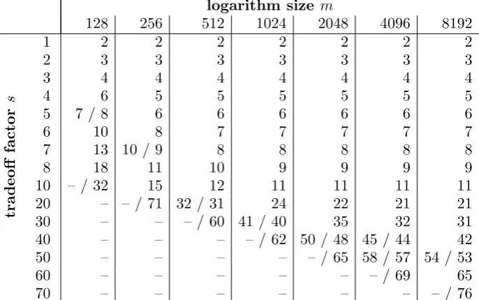
To estimate nas a function ofmand s, and to verify the estimates in simulations, we fix q= 0.99 and consider the hard cased= 2m−1.
For relevant combinations of m and s, we let ` = dm/se, fix N = 106 when estimating Re, and record the smallest n > s for which the volume quotient v < 2.
For some m and s, we verify the estimate by sampling M = 103 sets of n pairs
{(j1, k1), . . . , (jn, kn)} and solving each set for dwith the post-processing algorithm.
If d is thus recovered, the verification succeeds, otherwise it fails. We record the smallest n > s such that at most M(1−q) = 10 verifications fail.
logarithm size m
128 256 512 1024 2048 4096 8192
tradeoff
factor
s
1 2 2 2 2 2 2 2
2 3 3 3 3 3 3 3
3 4 4 4 4 4 4 4
4 6 5 5 5 5 5 5
5 7 / 8 6 6 6 6 6 6
6 10 8 7 7 7 7 7
7 13 10 / 9 8 8 8 8 8
8 18 11 10 9 9 9 9
10 – / 32 15 12 11 11 11 11
20 – – / 71 32 / 31 24 22 21 21
30 – – – / 60 41 / 40 35 32 31
40 – – – – / 62 50 / 48 45 / 44 42
50 – – – – – / 65 58 / 57 54 / 53
60 – – – – – – / 69 65
70 – – – – – – – / 76
Table 1: The estimated (A) and simulated (B) number of pairs nrequired foru
to be the closest vector tovinLallowingdto be recovered via Babai’s algorithm. If A = B, we only print A, otherwise we print B/A. Dash indicates no information.
Table 1 was produced by executing these procedures. To reduce the lattice bases, the block Korkin-Zolotarev (BKZ) algorithm, introduced by Schnorr [4, 5], was em-ployed, as implemented in fpLLL 5.2, with default parameters and a block size of min(10, n+ 1) for all combinations ofm,sandn. For these parameter choices, a basis takes at most minutes to reduce and solve for din a single thread.
variation becomes stronger when the factor whereby v increases or decreases for each increment of decrement of n is small in relation to two.
Compared to the processing algorithm originally proposed, the new post-processing algorithm efficiently achieves considerably better tradeoffs with practical time complexity for cryptographically relevant parameter choices. It furthermore re-quires considerably fewer quantum algorithm runs. Asymptotically, the number of runs required n tends to s+ 1 as m tends to infinity for fixed s, when we require a solution to be found without enumerating the lattice.
4.4 Further improvements
Above, we fixed a high minimum success probabilityq = 0.99 and considered the hard case whered= 2m−1. Furthermore, we required that mappingvto the closest vector inL should yield uwithout having to enumerate vectors in L.
In practice, some of these choices may be relaxed: Instead of requiring u to be the closest vector to vinL, we may enumerate all vectors in a hypersphere of limited radius centered on v. In cryptographic applications, the logarithm d may in general be assumed to be randomly selected on 2m−1 ≤d <2m. If not, the logarithm may be
randomized; solve x[c]g ford+c with respect to the basis g.
Other options include selectingmslightly greater than the bit length ofd, excluding subsets of pairs (j, k) from the lattice to eliminate pairs with large |α(j, k)|, and centering daround zero by admitting negative logarithms.
5
Summary and conclusion
We have introduced a new efficient post-processing algorithm that is practical for greater tradeoff factors, and in general requires considerably fewer quantum algorithm runs, than the original post-processing algorithm. To estimate the number of runs required, we have analyzed the probability distribution induced by the quantum algo-rithm and developed a method of simulating the quantum algoalgo-rithm.
With the new post-processing, our quantum algorithm achieves an advantage over Shor’s algorithms, not only in each individual run, but also overall, when targeting cryptographically relevant instances of RSA and Diffie-Hellman with short exponents, depending on how parameters are selected. The reader is referred to appendix A for a detailed analysis and quantification of the advantage.
Acknowledgments
I am grateful to Johan H˚astad for valuable comments and advice, to Lennart Bryniel-sson, and other colleagues, for their comments on early versions of this manuscript, and to past reviewers. Funding and support for this work was provided by the Swedish NCSA that is a part of the Swedish Armed Forces.
References
[1] L. Babai, On Lov´asz’ lattice reduction and the nearest lattice point problem,
Combinatorica 6(1) (1986), 1–13.
[2] M. Eker˚a,Modifying Shor’s algorithm to compute short discrete logarithms, IACR ePrint Archive, report 2016/1128 (2016).
[3] M. Eker˚a and J. H˚astad, Quantum algorithms for computing short discrete loga-rithms and factoring RSA integers, in: PQCrypto, Lecture Notes in Comput. Sci. 10346, Springer, Cham (2017), 347–363.
[4] C.-P. Schnorr, A hierarchy of polynomial time lattice basis reduction algorithms,
Theoret. Comput. Sci.53(2—3) (1987), 201–224.
[5] C.-P. Schnorr and M. Euchner, Lattice basis reduction: Improved practical algo-rithms and solving subset sum problems,Math. Program.66(1–3) (1994), 181–199.
[6] J.-P. Seifert, Using fewer qubits in Shor’s factorization algorithm via simultaneous Diophantine approximation, in: CT-RSA, Lecture Notes in Comput. Sci. 2020, Springer, Berlin Heidelberg (2001), 319–327.
[7] P.W. Shor, Algorithms for Quantum Computation: Discrete Logarithms and Fac-toring, in: SFCS, Proceedings of the 35th Annual Symposium on Foundations of Computer Science, IEEE Computer Society, Washington, DC (1994), 124–134.
[8] P.W. Shor, Polynomial-time algorithms for prime factorization and discrete loga-rithms on a quantum computer, SIAM J. Comput.26(5) (1997), 1484–1509.
[9] NIST, SP 800-56A:Recommendation for Pair-Wise Key-Establishment Schemes Using Discrete Logarithm Cryptography, 3rd revision. (2018)
[10] D. Gillmor, RFC 7919: Negotiated Finite Field Diffie-Hellman Ephemeral Param-eters for Transport Layer Security (TLS), (2016)
[11] T. Kivinen and M. Kojo, RFC 3526: More Modular Exponentiation (MODP) Diffie-Hellman groups for Internet Key Exchange. (2003)
A
Our advantage
In this appendix, we analyze our algorithm’s advantage when targeting RSA or the Diffie-Hellman key exchange scheme in safe-prime groups with short exponents.
A.1 Diffie-Hellman
The portions of the FIPS 800-56A recommendation [9] that pertain to Diffie-Hellman key exchange in G⊂F∗p were recently revised by NIST.
Migrating from Schnorr groups to safe-prime groups with full length exponents would result in a significant performance penalty. NIST therefore permits the use of short exponents; the exponent length m must be on 2z ≤ m ≤ dlog2re, where z is strength level of the group andr = (p−1)/2 is the group order.
strength in each run overall
dlog2pe levelz m s n v #ops adv #ops adv
2048 112 224 1 1 1.3·10
3 672 6.1 672 6.1
224 7 10 6.5·10−4 288 14.2 2880 1.4
3072 128 256 1 1 1.3·10
3 768 8.0 768 8.0
256 8 11 2.4·10−1 320 19.2 3520 1.7
4096 152 304 1 1 1.3·10
3 912 9.0 912 9.0
304 9 12 4.8·10−1 372 22.0 4464 1.8
6144 176 352 1 1 1.4·10
3 1056 11.6 1056 11.6
352 10 13 4.5·10−2 424 29.0 5512 2.2
8192 200 400 1 1 1.3·10
3 1200 13.7 1200 13.7
400 11 14 7.5 474 34.6 6636 2.5
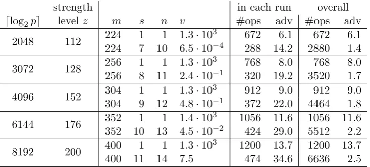
Table 2: Sample estimates for the complexity of computing short discrete loga-rithms in the FIPS 800-56A groups originally developed for TLS and IKE.
In Table 2 we provide estimates of the complexity of computing short discrete logarithms in these widely used safe-prime groups. The estimates were computed as in Section 4.3, for maximald= 2m−1 and≥99% success probability, except that we accept to enumerate vectors in L. We tabulate m, s and n, for s= 1, and for s the greatest tradeoff factor such that n−s≤3 with v close to two.
The number of group operations that need to be computed, in each run of the quantum algorithm, and overall in n runs, are tabulated for each tuple m, s and n, along with our advantage, defined as the fraction between 2dlog2re, the number of group operations in each run of Shor’s algorithm [2,7,8] for general discrete logarithms, and the number of group operations, in each run or overall, in our algorithm. We assume that standard double-and-add exponentiation is used.
Note that the latter comparison is quite generous to Shor as our algorithm has
≥99% probability of recoveringdafternruns. Multiple runs of Shor’s algorithm may be required to achieve a similar bound on the success probability.
As may be seen in Table 2, our algorithm reduces the number of group operations in each run by up to a factor of 34.6 for thesem,sandn. It provides an advantage, not only in each run, but also overall, even for large tradeoff factors, due to the new post-processing algorithm being more efficient and requiring fewer runs. We have verified the estimates by post-processing simulated outputs.
A.2 RSA
Let p, q >2 be two large distinct primes of length l bits. Then N =pq is said to be an RSA integer. To factorN intop and q, we propose to do the following:
Pick a random element g ∈ Z∗N. Let r denote the unknown order of g. Let ˜
p = (p−1)/2 and ˜q = (q−1)/2. Then r divides 2˜pq /˜ gcd(˜p,q˜). Let f(N) = (N −
d = f(N) mod r = ˜p+ ˜q −2l−1, assuming r > 2l−1, so the discrete logarithm d is short. To factor N, it hence suffices to compute dusing our algorithm, and to solve
p+q= 2(d+ 2l−1+ 1) andpq=N forpand q.
Recall that in our algorithm for computing short discrete logarithms [3], we require
d to be on 0 ≤ d < 2m, which implies m = l −1. Furthermore, we require r ≥
2`+m+ 2`d, where `=dm/se fors an integer. This implies s≥ 2 if the requirement that r≥2`+m+ 2`dis to be respected with high probability.
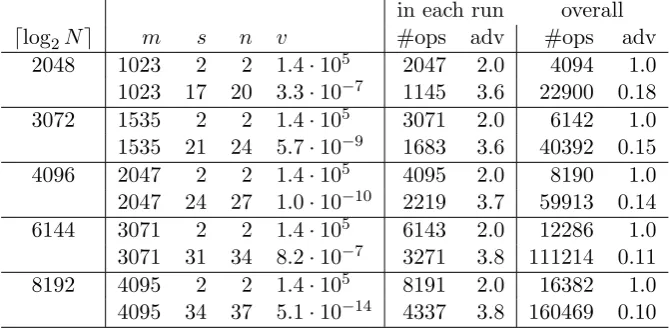
In Table 3 we provide estimates of the complexity of factoring RSA integers. The estimates were computed as described in Section 4.3, for ≥ 99% success probability and maximal d= 2m−1. Note that selecting d maximal slightly over-estimates the
hardness of factoring random RSA integers. We tabulate m, sand n, for s= n= 2, and for s the greatest tradeoff factor such thatn−s≤3 whilst keepingv sufficiently small to avoid having to enumerate the lattice.
The estimates are tabulated as described in Section A.1, except that we compute our advantage in relation to a single run of Shor’s order finding algorithm. We have verified the estimates by post-processing simulated quantum algorithm outputs.
in each run overall
dlog2Ne m s n v #ops adv #ops adv
2048 1023 2 2 1.4·105 2047 2.0 4094 1.0 1023 17 20 3.3·10−7 1145 3.6 22900 0.18 3072 1535 2 2 1.4·105 3071 2.0 6142 1.0 1535 21 24 5.7·10−9 1683 3.6 40392 0.15 4096 2047 2 2 1.4·105 4095 2.0 8190 1.0 2047 24 27 1.0·10−10 2219 3.7 59913 0.14 6144 3071 2 2 1.4·105 6143 2.0 12286 1.0 3071 31 34 8.2·10−7 3271 3.8 111214 0.11 8192 4095 2 2 1.4·105 8191 2.0 16382 1.0 4095 34 37 5.1·10−14 4337 3.8 160469 0.10
Table 3: Estimated complexity of factoring RSA integers with ` = dm/se and
s≥2 in multiple runs, with≥99% success probability and maximald= 2m−1.
As may be seen in Table 3, we obtain an advantage in each run of the algorithm, that translates into a reduction of the size and depth of the quantum circuit.
For s = 2, we perform the same number of operations overall in the two runs, as Shor’s algorithm does in a single run. Hence, the benefit of reduced circuit size and depth in each individual run comes at no cost in terms of the overall number of operations that need to be performed. For s > 2, we obtain a greater advantage in each individual run of the algorithm, at the expense of performing a greater number of operations overall than Shor’s algorithm does in a single run.
A.2.1 Breaking RSA with an advantage in a single run
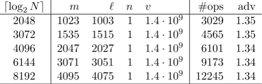
When using the new post-processing algorithm, we may let `=m−δ for some small
δ, instead of letting ` =dm/se for s an integer. This tweak allows us to remove the obstacle that prevented us from achieving an advantage over Shor’s algorithm in a single run above, without affecting the analysis of the algorithm.
Experiments, in which we select random N =pq and estimate the distribution of orders of elementsgselected uniformly at random fromZ∗N by partially factoringp−1
andq−1, indicate that selectingδ = 20 results in a very high probability of respecting the requirement that r≥2`+m+ 2`d.
dlog2Ne m ` n v #ops adv
2048 1023 1003 1 1.4·109 3029 1.35 3072 1535 1515 1 1.4·109 4565 1.35 4096 2047 2027 1 1.4·109 6101 1.34 6144 3071 3051 1 1.4·109 9173 1.34 8192 4095 4075 1 1.4·109 12245 1.34
Table 4: Estimated complexity of factoring RSA integers with ` = m−δ for
δ= 20 in a single run, with≥99% success probability and maximald= 2m−1.
In Table 4 we provide estimates for the complexity of factoring RSA integers in a single run of our quantum algorithm with ` = m−δ for δ = 20. As evidenced, tweaking `enables us to achieve an advantage over Shor’s order finding algorithm in a single run, at the expense of enumerating a moderate number of lattice vectors.