The Peano-series solution for modeling shear horizontal waves in piezoelectric plates

The Peano-series solution for modeling shear horizontal

waves in piezoelectric plates

I. Ben Salah1a, A. Njeh1 and M.H. Ben Ghozlen1

1

Laboratoire de Physique des Matériaux, FSS, BP 1171, 3000 Sfax, Tunisie

Abstract. The shear horizontal (SH) wave devices have been widely used in electro-acoustic. To improve their performance, the phase velocity dispersion and the electromechanical coupling coefficient of the Lamb wave should be calculated exactly in the design. Therefore, this work is to analyze exactly the Lamb waves polarized in the SH direction in homogeneous plate pie.zoelectric material (PZT-5H). An alternative method is proposed to solve the wave equation in such a structure without using the standard method based on the electromechanical partial waves. This method is based on an analytical solution, the matricant explicitly expressed under the Peano series expansion form. Two types of configuration have been addressed, namely the open circuited and the short circuited. Results confirm that the SH wave provides a number of attractive properties for use in sensing and signal processing applications. It has been found that the phase velocity remains nearly constant for all values of h/λ (h is the plate thickness, λ the acoustic wavelength). Secondly the SH0 wave mode can provide very high electromechanical coupling. Graphical representations of electrical and mechanical amounts function of depth are made, they are in agreement with the continuity rules. The developed Peano technique is in agreement with the classical approach, and can be suitable with cylindrical geometry.

1 Introduction

As is well known for development of acousto-electronic devices the electro-mechanical coupling

coefficient (K2) of acoustic wave has a great importance. In this connection one of the modern lines

of investigation in acoustics is the search of such wave types for which the value of K2 is maximal.

At present there exist the papers showing that fundamental shear-horizontal (SH0) acoustic waves in

thin (in comparison with wavelength) piezoelectric plates possess by significantly more electromechanical coupling coefficient than surface acoustic waves (SAW) in the same material [1-3].

This paper presents a detailed investigation of acoustic waves propagating in piezoelectric plates. The material selected for our study was Zirconium Titanate de Plomb (PZT-5H). This material was selected since it is a strong piezoelectric material that is widely used for surface acoustic wave (SAW) devices [4]. In particular, the waves of interest here are the so-called SH (shear-horizontal) acoustic waves. The SH wave has a single component of particle displacement that lies in the plane

e-mail : bs_issam@yahoo.fr

EPJ Web of Conferences DOI: 10.1051/

C

Owned by the authors, published by EDP Sciences, 2012 ,

epjconf 20122/

of the plate surface and is at right angles to the direction of wave propagation. One of the attractive properties of such a wave is that the component of particle displacement normal to the free surface is zero. The absence of a surface normal component allows the wave to propagate in contact with a liquid without coupling and the energy leaking into the surrounding fluid can be ignored. SH wave devices can therefore be used for measuring properties of liquids and in liquid-phase-based sensors

[5, 6]. In such a plate the fundamental wave mode, namely shear horizontal (SH0) mode can

propagate, while the higher order modes are cut off [7]. The data presented in this paper is essential for the proper design of various devices based on acoustic waves propagating in PZT-5H plates.

The aim of this paper is to study the propagation behaviour of such SH wave in homogeneous

plate piezoelectric material for which the value of K2 is maximal. The resolution of the problem

passes by the analytical formulation generally proceeding from the propagator matrix M, representing the matricant solution of the governing ordinary differential system [8]. A conventional way of the numerical treatment relies on the discretization (Thomson–Haskell) method, computing

M as the product of exponentials of the piecewise homogeneous system matrix Q. This method has

been further improved in [9–11]. Discussion of some other numerical methods may be found in [12].

2 Theoretical analysis

We consider the propagation of acoustic waves in a plate of arbitrary piezoelectric material. The

geometry of the problem under consideration is shown in Figure 1. Waves propagate along the x1

direction of a piezoelectric plate bounded by planes x3 = 0 and x3 = −h. The plate presents material

symmetries which allow to decouple the SH waves (Shear Horizontal) polarized along x2-axis. For

illustration a piezoelectric plate PZT-5H assumed hexagonal has been adopted. Table 1 show the elastic and electric proprieties of the piezoelectric plate.

Fig. 1.The geometry of the problem and coordinate system used to analyze propagation of acoustic waves in a piezoelectric plate.

Table 1. Elastic and electrical properties of piezoelectric plate (PZT-5H) [4]

C11=C22 (GPa) C12 (GPa) C13=C23 (GPa) C33 (GPa) C44=C55 (GPa)

151 98 96 124 23

e31=e32(C/m²) e33(C/m²) e15=e24(C/m²) εεεε11(C/Vm) εεεε33(C/Vm)

-5.1 27 17 15×10-9 13.27×10-9

The system of governing equations involves the equation of motion, the Maxwell equation in the quasi-static approximation and the piezoelectric constitutive equations:

Wave propagation

x1

x

x

h

SH

0 , , = = j i j ij i D T u&&

ρ

In these equations, ρ density and Cijkl the tensors of elastic, eijk is the piezoelectric constants and

εik is the dielectric constants.

To describe the SH waves in homogeneous plate piezoelectric material, the following boundary and continuous conditions should be satisfied. It should be pointed out that two kinds of electrical boundary conditions, electrically open and shorted conditions, would be taken into account in this

study. It must be reminded that the generalized stress vector T includes mechanical stress vector ti3

(i=2) and the normal electrical displacement D3, in the same way the generalized displacement

vector U includes the mechanical displacement ui (i=2) and the electrical potential φ. Both surfaces

of the plate x3 = 0 and x3 = -h

t23 = 0 at x3 = 0 and x3 = - h

Electric short case: φ = 0 (3)

Electric open case: σ = 0 (4)

σ refers to the charge density, it can be deduced from D3 values in the neighborhood of the both

surfaces ) ( ) ( ₃ 3 − + _{− −} −

=D h D h

σ

According writing of the constitutive equations and the motion equation (1), the wave equation becomes a matrix system expressed using the Thomson-Haskell parameterization of the Stroh

formalism [13], with η (x3) = [U, T]T ; U = [iωu, iωφ]T and T = [ti3, D3]T :

), ( ) ( )

( _{3 3 3}

3 x x Q i x dx d η ω

η =

where the 4-component state vector η (x3) comprises the amplitudes of (6).

The general solution for the state vector can be written as:

)] ( exp[ ) ( ) , ,

(x₁ x₃ t η x₃ i k₁x₁ ωt

η = −

Where ω is the angular frequency, k1 is the projection on x1 axis of the wave vector and ω=2πf is the

frequency.

The explicit solution reveals the Peano expansion of the matricant. The wave equation thus

formulated has an analytical solution expressed between a reference point (x1; 0; x03) and some point

of the plate (x1; 0; x3) in the propagation plane. This solution is called the matricant and is explicitly

written under the form of the Peano series expansion [14 - 16]:

∫

∫

∫

( _{3 3}0 2 x _{1 1}

x x

x

x Q d i Q Q d d

i I x x

M _{ω ξ ξ ω ξ} ξ _{ξ ξ ξ} K

where I is the identity matrix of dimension (4×4). If the matrix components Q(x3) are bounded in the

study interval, these series are always convergent [17]. The components of the matrix Q are

continuous in x3 and the study interval is bounded (thickness of the waveguide), consequently the

hypothesis is always verified.

Boundary conditions: Using the propagator property of the matricant through the plate thickness,

the state-vector (defined in (6)) at the second interface η (-h) is evaluated from the state-vector at the

first interface η (0) as follows:

0 22 21

12 11

         

 

=

     

− T

U

M M

M M

T U

h

where η (0) is a vector of ‘initial’ conditions on U and T at x3 = 0, and M11, . . . ,M22 are the 2 × 2

blocks of M (-h,0).

The aim is to seek out the zeros of the determinant of M21 (2×2), that leads to find the couples of

values (kx, ω) which describe the dispersion curves. To calculate the dispersion curves, we evaluate

numerically the matricant M (-h, 0) from the expression (8). This step requires us to truncate the Peano series and to numerically calculate the integrals. Thus, the error can be estimated and controlled [17]. For the calculations in the plate we retained 9 terms in the series and evaluate the integrals over 100 points using the Simpson’s rule.

These choices are not optimized but ensure the convergence of the solution and the accuracy of

the results in the range of values h/λ considered for a reasonable computation time.

3 Results and discussions

In a plate of a particular thickness h, an infinite number of modes can propagate for each allowed type of wave. The velocity of each mode can be calculated as a continuous function of either the

thickness-to wavelength ratio h/λ for two cases of polarizations open and short circuited “OC” and

“SC”. It can be seen that the SH0 mode has negligible velocity dispersion. The phase velocity nearly

constant for all values of h/λ. Figure 2 shows that there is one all-pass mode, it can propagate at any

frequency, while all the other modes are high-pass modes. It can be seen from Figure 2 that the

lowest-order SH0 wave is nearly dispersion less. The velocity of this mode lies within 2370 ± 3.5 m

s−1 for all values of h/λ. The fact that the velocity remains nearly constant is a great advantage in the

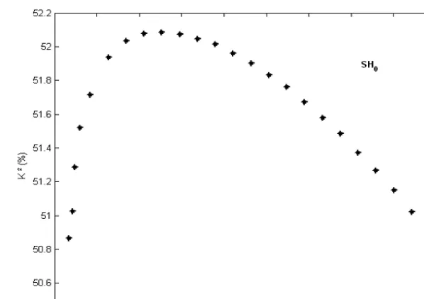
design of wide-bandwidth devices [18]. The electromechanical coupling coefficient of the SH mode

calculated from equation K2 = 2 (VOC− VSC) / VOC is shown in Figure 3. We note that K

2

reaches a

value as high as 52.09% for h/λ = 0.0253. This is nearly eight times the value of K2 for SAWs in the

widely used strong piezoelectric material PZT-5H. Due to its large coupling coefficient, devices based on this wave can operate efficiently over a wide bandwidth [18].

Fig. 3.Electromechanical coupling coefficient K2 as a percentage as a function of h/λ for the SH0 mode.

The stress and mechanical displacement distribution in PZT-5H plate will be taken into account

for fundamental mode SH0 at a frequency of 0.06 MHz with h/λ = 0.0253. The variation of the

mechanical displacement U2 and the stress component T23 with respect to x3/h, for SH0 mode are

shown in Figure 4 for electrically open. As well, the variation of the electrical displacement D3 and

electrical potential φ with depth are reported in Figure 5 for electrically open. The obtained plots are

in agreement with continuity rules and the free character of the lower and upper surfaces of the plate.

The representation of displacement component U2, concerning the SH0 mode, shows that the

coupling is strong when the mechanical displacement parallel to the piezoelectric axis is of great amplitude for all points of the same section of the plate (Figure 4-a).

The obtained numerical results are coherent with standard methods [9, 10, 17]. The advantage of the Peano expansion method becomes essential for inhomogeneous materials and cylindrical geometry.

Fig. 4. Variation of normalized SH0 mechanical component U2 and T23 for different values of x3/h for both surfaces unmetallized (OC)

-1 -0.9 -0.8 -0.7 -0.6 -0.5 -0.4 -0.3 -0.2 -0.1 0 -0.2

0 0.2 0.4 0.6 0.8 1 1.2

x₃/h

N

o

rm

a

liz

e

d

m

e

c

h

a

n

ic

a

l

d

is

p

la

c

e

m

e

n

t

u2

real (u2)

imag (u₂)

-1 -0.9 -0.8 -0.7 -0.6 -0.5 -0.4 -0.3 -0.2 -0.1 0 -1

-0.8 -0.6 -0.4 -0.2 0 0.2 0.4 0.6 0.8 1

x₃/h

N

o

rm

a

liz

e

d

s

tr

e

s

s

c

o

m

p

o

n

e

n

t

T23

real (T₂₃) imag (T₂₃)

(a) (b

Fig. 5. Variation of normalized SH0 electrical component φ and D3 for different values of x3/h for both surfaces unmetallized (OC)

4 Conclusion

This paper has presented a detailed investigation of shear- horizontal acoustic waves in plates of

PZT-5H. The SH wave can provide very high electromechanical coupling. For example, value of K2

as high as 52.09% can be obtained for SH waves propagating along the x2-axis of PZT-5H plate. The

nearly nondispersive propagation and high value of K2 make this wave attractive for use in a variety

of signal processing and sensing applications. The SH wave can also be advantageously employed in liquid-phase-based chemical and biological sensors [19]. In order to operate at high efficiency, SH wave devices need plates much thinner than the acoustic wavelength.

References

1. B. D. Zaitsev, S. G Joshi., I. E. Kuznetsova, IEEE Trans. Ultrason. Ferroel. and Freq. Control

46, 1298-1302 (1999).

2. I. E. Kuznetsova, B.D. Zaitsev, S.G. Joshi, I.A. Borodina, IEEE Trans. Ultrason. Ferroel. And

Freq. Control. 48, 322 – 328 (2001).

3. I. E. Kuznetsova, B.D. Zaitsev, S.G. Joshi, I.A. Borodina, Electronic Letters 34, N23.2280-

2281 (1998).

4. K. Anil, D. Chakraborty, Mater. Des. 30, 1216-1222 (2009).

5. T.M. Niemczyk, S.J. Martin, G.C. Frye, A.J. Ricco, J. Appl. Phys. 64, 5002–8 (1988).

6. S.J. Martin, A.J. Ricco, T.M. Niemczyk, G.C. Frye, Sensors Actuators 20, 253–68 (1989).

7. B.D. Zaitsev, S.G. Joshi, I.E. Kuznetsova, Smart Mater. Struct. 739–744 (1997).

8. M.C. Pease III, Methods of Matrix Algebra, Academic Press, New York, (1965).

9. S.I. Rokhlin, L. Wang, J. Acoust. Soc. Am. 112, 822–834 (2002).

10. B. Hosten, M. Castaings, Ultrasonics 41, 501–507 (2003).

11. Eng Leong Tan, J. Acoust. Soc. Am. 119, 45–53 (2006).

12. G.R. Liu, Z.C. Xi, CRC Press, Boca Raton, FL, (2002).

13. A. N. Stroh, Journal of Mathematics and Physics 41, 77–103 (1962).

14. F. Gantmacher, the theory of matrices (Wiley Interscience) (1959).

15. G. Peano, Mathematische annallen 32, 450–456 (1888).

16. M. Pease, Methods of matrix algebra (Academic Press) (1965).

17. C. Baron, Thesis, Université Bordeaux 1 (2005).

18. K. Michio, A. Junya, H. Hideya, I. Mamoru, Jap. J. A. Phy., 40, 3722 (2001).

19. F. Josse, F. Bender, W. Richard, Anal. Chem., 73 (24), 5937–5944 (2001).

-1 -0.9 -0.8 -0.7 -0.6 -0.5 -0.4 -0.3 -0.2 -0.1 0 -0.2

0 0.2 0.4 0.6 0.8 1 1.2

x3/h

N

o

rm

a

liz

e

d

e

le

c

tr

ic

a

l

p

o

te

n

ti

a

l

φ

real (φ) imag (φ)

(a)

-1 -0.9 -0.8 -0.7 -0.6 -0.5 -0.4 -0.3 -0.2 -0.1 0 -1

-0.8 -0.6 -0.4 -0.2 0 0.2 0.4 0.6 0.8 1

x3/h

N

o

rm

a

liz

e

d

e

le

c

tr

ic

a

l

d

is

p

la

c

e

m

e

n

t

D3