NNLO QED contribution to the
µ
e
→
µ
e
elastic scattering
Jonathan Ronca1,a b
1Instituto de Física Corpuscular, Universitat de València, Consejo Superior de Investigaciones Científicas, Parc Científic, E-46980 Paterna, Valencia, Spain
Abstract. We present the current status of the Next-to-Next-to-Leading Order QED contribution to theµe -scattering. Particular focus is given to the techniques involved to tackle the virtual amplitude and their automatic implementation. Renormalization of the amplitude will be also discuss in details.
1 Introduction
The current measurements of the muon anomalous mag-netic momentaµ = (gµ−2)/2 indicate a discrepancy of
∼3.5σfrom the Standard Model prediction [1]. This fact might be a hint of new physics. New upcoming experi-ments at Fermilab and J-PARC will improve significantly the precision ofaexpµ , hence higher accuracy forathµ from
the theoretical side is required.
A very clean way to achieve the aimed precision in-volves the determination of the leading hadronic contri-bution ∆αhad(q2) to the electromagnetic coupling in the
space-like region [2, 3]. TheMUonE experiment, recently proposed at the CERN, is meant to obtain an estimation of ∆αhad(q2) through a measurement of the differential cross
section of theµe-elastic scattering. In order to be com-petitive with the time-like datas, a precision of 10ppm is required, both on statistical and systematic errors.
QED contributions to µe-elastic scattering constitute an irreducible background for the measurement, and they represent a relevant source of systematic errors; results for Leading Order (LO) and Next-to-Leading Order (NLO) corrections are already available [4], as well as the Next-to-Next-to-Leading Order (NNLO) hadronic ones [5, 6]. However, Next-to-Next-to-Leading Order (NNLO) cor-rections toµe-elastic scattering are mandatory to achieve the 10ppm precision.
In this work, we summarize the current status of the double-virtual contributions to the NNLO QEDµe-elastic scattering. The review is organized as follows: Section 2 recaps the external kinematic definitions we use for char-acterizing theµe-elastic scattering; Section 3 states the ba-sics of the calculation process, stressing the importance of theFeynman integrals. The next sessions will present the heart of this calculation: thedecompositionof the ampli-tude and the evaluation of themaster integrals.
aBased on a collaboration with S. di Vita, S. Laporta, P. Mastrolia, M.
Passera, T. Peraro, A. Primo, U. Schubert and W.J. Torres Bobadilla.
be-mail: [email protected]
The decomposition strategies are presented in Section 4. We discuss the main features of the Adaptive Inte-grand Decomposition [7, 8] and its implementation Aida [9, 10], and the Integral Reduction algorithms involving theIntegration-by-parts identities[11–14]. These method are exploit to obtain a reduction of the full amplitude in terms of a minimal set of master integrals. Section 5 is fo-cused on the evaluation approaches, presenting the analyt-ical and the numeranalyt-ical ways. Analytanalyt-ical strategy is based on solvingsystems of differential equations[15–17] which master integrals obey. The main results of the analyti-cal method for theµe-elastic scattering are collected into [18, 19], and cross-checked numerically. Alternatively, a numerical method which can be userful in these calcula-tion is the so-calledsector decomposition[20], which will be briefly introduced.
Section 6 is devoted to present the complete Mathe -maticaimplementation which embeds each step of the cal-culation, from the generation of the amplitude to evalu-ation of the master integrals. A flowchart of the global algorithm is presented in Fig. 2.
In Section 7 we define the renormalization procedure which will be adopted to obtain a UV finiteµe-elastic Scat-tering Amplitude. Both MS andon-shellschemes are em-ployed to renormalize respectively the QED coupling con-stant and the muon fermion field and mass.
Lastly, we present the main result achieved for theµe -elastic scattering and we point out the next steps needed to complete the full NNLO contribution.
2
µ
e
-elastic Scattering process
The process under investigation is the elastic scattering
µ+(p1)e−
(p2)→e−(−p3)µ+(−p4), (1)
where pi are the on-shell momenta: p21 = p 2 4 = m
2 µ
and p2 2 = p
2 3 = m
2
si j=(pi+pj)2, define
s=s12, t=s23, u=s13,
s+t+u=2m2e+2m2µ. (2)
The physical phase-space region is constrained by the fol-lowing conditions
s≥(me+mµ)2,
−λ(s,m
2 µ,m2e)
s <t<0, λ(s,m2µ,m2e) =s
2+
(m2µ)2+(m2e)
2−
2sm2µ
−2sm2e−2m
2
em
2 µ.
(3)
The ratio between electron and muon mass is of the order 10−5. This enforce the validity of the massless elec-tron approximation, which yields many advantages to the NNLO calculation. Therefore, from now on we setme=0 andmµ=m.
3 Double-virtual contributions
Within the perturbative QFT approach, the QED cross sec-tionσof theeµ-scattering is a series expansion in terms of the coupling constantα,
σ=σLO+σNLO+σNNLO+· · ·+O(α2+n). (4)
For 2→2 scattering process,σis also related to the Feyn-man amplitudeMthrough the well-known relation
σ=Cflux Z
|M|2dPS2, (5)
whereCfluxis the flux factor anddPS2is the infinitesimal
phase-space element. Matching Eq. (4) and (5), the order-by-order expression ofσis manifest,
σLO∼ |M0|2,
σNLO∼2Re[M∗0M1l]+|Mr|2, σNNLO∼2Re[M∗0M2l]+2Re[M∗1lM1l]
+2Re[M∗rM1l,r]+|M2r|2,
(6)
whereM0is the Born amplitude,M1landM2lare respec-tively the one and two-loop Feynman amplitude,Mr and
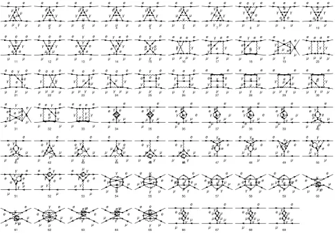
M2rare the real and the double-real emission amplitudes, with respectively one and two more particles emitted in the final state, andM1l,rthe real-virtual amplitudes, one-loop amplitude with one more particle emitted in the final start. The double-virtual contributionM2ltoσNNLO(Fig. 1) is a combination of dimensionally regularizedFeynman in-tegrals
2Re[M∗0M2l]=
X
¯
i
A¯iIi(s), (7)
where the coefficients A¯i depend on the kinematic vari-abless=(s,t,m2). The Feynman integrals1I
i(s) have the general form
Ii(s)= Z
k
N¯i(k,s)
Di1
1 · · ·D
in
n
, ¯i∈Nn, (8)
1R
k=
R
M ddk1 (iπd/2)
ddk2
(iπd/2), andk=(k1,k2)
and depend on the kinematic invariants s and the di-mension d. The numerator N¯i is a general polynomial of the scalar products between loop and external mo-menta. The denominatorsDj are inverse scalar propaga-tors, whose form isDj=qj(k,p)2−m2j. The multi-index ¯
i = (i1,· · · ,in) contains the exponents of the denomina-tors.
Direct integration of Feynman integrals objects is usu-ally not allowed. A viable way to calculate them effi -ciently involves decomposition methods: Feynman grals can be expressed into combinations of "simpler" inte-grals. Such integrals can be evaluated either analytically of numerically. In the next session, the algorithm employed in the calculation of the amplitude (7) is presented.
4 Decomposing the Amplitude
There exist several decomposition methods, which can be apply either to integrands[21–23] or integrals[11, 24–26]. An optimized algorithm to achieve a complete decompo-sition of a Feynman integrals will involve both methods.
4.1 Adaptive Integrand Decomposition
As extensively discussed in [7, 8], theAdaptive Integrand Decomposition (AID) is an algorithm that works at inte-grand level. It exploits the (rational and) polynomial struc-ture of the integrand in order to achieve an iterative decom-position of the numerator.
The basic ingredient is the splitting of the d -dimensional space intoparallelandtransversecomponent [27] w.r.t. the space spanned by the independent external momenta:
d=dk+d⊥ =⇒ kαi =k
α
ki+λ
α
i. (9)
It can be shown that Eq. (9) makes the polynomial struc-ture of the integrand manifest, and liable to perform poly-nomial division without passing by the Gröbner basis
[28]. Therefore, the numerator can be written as
N¯i(k,s)= n
X
j=1
N¯i−e¯j(k,s)Dj+ ∆¯i−e¯j(k,s), e
j k=δ
j k. (10)
The polynomial division can be iterated for every
N¯i−e¯j(k,s). After the complete division of the numerator,
the integrand is cast into the following form
N¯i(k,s)
Di1
1 · · ·D
in
n =
|i|
X
|j|=0 X
¯j
∆¯j(k,s)
Dj1
1 · · ·D
jn
n
. (11)
Theresidues∆¯j(k,s) are polynomials depending of the
ir-reducible scalar products, a minimal set of scalar product between loop and external momenta. Therefore, the total double-virtual amplitude can be cast into the form
2Re[M∗0M2l]=
X
¯
i
|i|
X
|j|=0 X
¯
j
A¯i
Z
k
∆¯j(k,s)
Dj1
1 · · ·D
jn
n
e μ e μ γ μ γ μ γ μ μ 1 e μ e μ γ μ γ e e γ e 2 e μ e μ γ μ γ μ μ γ μ 3 e μ e μ γ μ γ e e γ e 4 e μ e μ γ μ γ μ μ γ μ 5 e μ e μ γ γ μ μ γ μ μ 6 e μ e μ γ μ γ μ μ γ μ 7 e μ e μ γ e γ e γ e e 8 e μ e μ γ e γ e e γ e 9 e μ e μ γ e γ μ μ γ μ 10 e μ e μ γ e γ e e γ e 11 e μ e μ γ e γ μ μ γ μ 12 e μ e μ γ γ e e γ e e 13 e μ e μ γ e γ e e γ e 14 e μ e μ γ μ μ e e γ γ 15 e μ e μ γ μ μ e γ e γ 16 e μ e μ γ e e e γ μ γ 17 e μ e μ γ e e e γ μ γ 18 e μ e μ e e γ γ μ μ γ 19 e μ e μ γ e e γ μ μ γ 20 e μ e μ γ e γ e e γ μ 21 e μ e μ γ e e γ μ γ μ 22 e μ e μ γ e μ γ μ γ μ 23 e μ e μ e γ μ μ γ μ γ 24 e μ e μ γ e γ e e γ μ 25 e μ e μ e γ μ μ γ μ γ 26 e μ e μ γ e γ e γ e μ 27 e μ e μ e γ μ μ μ γ γ 28 e μ e μ e γ μ μ μ γ γ 29 e μ e μ e γ μ γ μ γ μ 30 e μ e μ γ e γ e μ γ μ 31 e μ e μ γ e γ e γ e μ 32 e μ e μ γ e e γ μ μ γ 33 e μ e μ γ γ e e γ e e 34 e μ e μ γ γ μ μ γ μ μ 35 e μ e μ γ γ e e e γ e 36 e μ e μ γ γ μ μ μ γ μ 37 e μ e μ γ γ e e e γ e 38 e μ e μ γ γ μ μ μ γ μ 39 e μ e μ γ γ μ μ e e γ 40 e μ e μ γ γ μ μ μ μ γ 41 e μ e μ γ μ γ μ γ μ μ 42 e μ e μ γ γ μ μ γ μ μ 43 e μ e μ γ γ μ μ μ γ μ 44 e μ e μ γ μ γe eγ μ 45 e μ e μ γ μ γ μ μ γ μ 46 e μ e μ γ γ e e e e γ 47 e μ e μ γ γ μ μe e γ 48 e μ e μ γ e γ e γ e e 49 e μ e μ γ γ e e γ e e 50 e μ e μ γ γ e e e γ e 51 e μ e μ γ e γe e γ e 52 e μ e μ γ e γ μ μ γ e 53 e μ e μ γ e e γ e μ γ 54 e μ e μ γ e μ μ γ μ γ 55 e μ e μ γ e μ γ e e γ 56 e μ e μ γ e μ γ μ μ γ 57 e μ e μ e γ e e γ μ γ 58 e μ e μ e γ μ μ γ μ γ 59 e μ e μ e γ e e γ γ μ 60 e μ e μ e γ μ μ γ γ μ 61 e μ e μ e γγ μ μ γ μ 62 e μ e μ e γ μ γ e e γ 63 e μ e μ e γ μ γ μ μ γ 64 e μ e μ γ e e γ e γ μ 65 e μ e μ γ γ γ e e e e 66 e μ e μ γ γ γ μ μ μ μ 67 e μ e μ γ γ γ μ μ e e 68 e μ e μ γ γ γ e e μ μ 69
Figure 1.Two-loop diagrams contributing the QED NNLO amplitude for theµe-scattering
AID has been successfully applied to many amplitude [7, 8, 10]. An automated Mathematicaimplementation of this algorithm has been developed, called Aida[9, 10]. It accepts the FeynArts[29] output (namely the complete unreduced amplitude) and perform the AID, exploiting the
finite fields reconstructionmade available through Finite -Flow[30]. Its output is finally translate into integral nota-tion.
4.2 Integration-by-parts identities
As a consequence of the d-dimensionality and the shift/rotational invariance of the Feynman integrals, an en-tire class of new relations [11] can be found:
Z
k
f(k)= Z
k
evµ ∂∂kµ f(k)
⇓
Z
k
∂
∂kµ[vµf(k)]=0,
(13)
where vµ can be either a loop or an external momenta. These identities between integrals are called Integration-By-Parts Identities(IBPs) [11, 12, 31]. Letting f(k) be the reduced integrands coming from AID,
Z
k ∂ ∂kµi
vµ ∆¯j(k,s) Dj1
1 · · ·D
jn n =0
. (14)
IBPs are employed to generate a large system of equalities, which are not all independent. As a consequence, there exists a minimal set of integrals which can not be reduced further: they are known as Master Integrals (MIs) [32]. The general expression for a MI is
Ti(s)= Z
k Ssi1
1 · · ·S
sim
m
Dri1
1 · · ·D
rin
n
, (15)
whereS1. . .Smare the irreducible scalar products. IBPs allow the ultimate decomposition of the Feynman integrals in the basis of MIs,
Z
k
∆¯j(k,s)
Dj1
1 · · ·D
jn
n =
NMIs
X
l=1
c¯jlTl(s), (16)
which amounts the complete double-virtual contribution in this simple form,
2Re[M∗0M2l]= NMIs
X
l=1 X ¯i
|i|
X
|j|=0 X
¯j
A¯ic¯jl
Tl(s).
= NMIs
X
l=1
ClTl(s).
(17)
"simplicity" criterion. Although Laporta MIs look simpler, they might be not the convenient choice if one wants to evaluate them analytically [17, 33, 34].
There exist several public codes [35–37] which can provide IBPs and the Laporta MIs for any input topology, such asreduze[13] andkira[14]. It is important to un-derline that these codes may accept as input a custom MIs basis; in this case, their output will be the IBPs expressed in terms of the chosen basis.
5 Evaluating the Master Integrals
The-expansion of MIs can be achieved by either analyti-cal or numerianalyti-cal evaluation. In this picture,d=4−2and the expansion reads
Ti(s)=
∞
X
k=−np kg
k(s), (18)
wherenpis the order of the higher order pole into theTi(s) series. In practice, the series expansion will be truncated to a finite order, such that every Feynman amplitude is expanded up toO(). Here, the evaluation strategies em-ployed in this calculation are presented.
5.1 Differential equations
The analytical approach exploits the IBPs to build a system of differential equation [15]:
∂ ∂sj
Ti(sj)=[A(,sj)]ikTk(sj)
=[A0(sj)+A1(sj)]ikTk(sj)
(19)
where the MIs basis is chosen in such a way that the matrix A(,sj) depends linearly on.
If there exist a rotation matrixR(sj) such that Eq. (19) can be cast into thecanonical form[16], simbolically ex-pressed as
Fi(sj)=[R(sj)]ikTk(sj) (20)
⇓
∂ ∂sj
Fi(sj)=[B(sj)]ikFk(sj) (21)
the PDE admits a solution in terms of theChen’s iterated integral
Fi(sj)=
Pe
R γdBj
ik
Fk(sj0) (22)
and its -expansion casts Fi(sj) to the form (18). The boundary conditionFk(sj0) are chosen by exploiting
reg-ularity conditions into the phase space appropriate kine-matic limits.
The matrixR(sj) can be found by means of the
Mag-nus exponential method[17, 38, 39], that provides a close
formula for the rotation matrix,
R(sj)=exp
h
Ω(sj,sj0) i
,
Ω(sj,sj0)=
∞
X
n=1
Ωn(sj,sj0),
Ω1(sj,sj0)= Z sj
sj0
dτ1A0(τ1),
Ω2(sj,sj0)=
1 2
Z sj
sj0
dτ1Z τ1
sj0
dτ2[A0(τ1),A0(τ2)].
(23)
The complete order-by-order expression forΩ(sj,sj0) can
be found in [17].
The PDE method is extensively discussed in [16, 40– 42], and if has been employed in the evaluation of several two-loop Feynman integrals [43–47], including the com-plete MIs basis for theµe-scattering (see [18, 19])
5.2 Sector decomposition
The alternative way to obtain (18) involves numerical methods.
A general algorithm valid for any multi-loop Feynman integral is the sector decomposition[20]. Briefly, Feyn-man parametrization appliedTi(s) changes the integration space from the Minkowski (or Euclidean) space to then -dimensional unit cube2Cn
Ti(s)=
Z
M
ddk fi(k)=
Z
Cn
dnxf˜i(x). (24)
The unit cubeCn can be iteratively decomposed and de-formed into multiple sub-domains, until the pole struc-ture of the integral manifests multiplicatively into the inte-grand,
Z
Cn
dnxf˜i(x)= n
X
j=1 Z
Cn dnx
ˆ
fi(x)
xaj−bj
j
, (25)
and subsequently isolated by means of theend-point sub-tractionmethod. Foraj=bj=1, such method reads
Z1
0
dxj
ˆ
fi(xj)
x1− j
= fˆ(0)
+
Z 1
0
dxj
ˆ
f(xj)−f˜(0)
x1− j
. (26)
Once the sector decomposition has been applied, MIs lie to the following form
Ti(s)=
∞
X
k=−np
n
X
j=1 k
Z
Cjk djkxf˜
i jk(x). (27)
The integrals appearing in Eq. (27) arefiniteand they can be integrated using numerical algorithms.
The integration on the physical phase-space region usually requires contour deformation procedures, such that the threshold singularities of the integrand can be avoided and the numerical stability is preserved.
The complete algorithm has been implemented into a code, SecDec [48]. It goes through the interation of the Sector Decomposition algorithm and performs the nu-merical evaluation using Monte Carlo integration methods available into the Cubalibraries [49], with the possibility of deform the integration contour.
6 Automation
A complete automation of the evaluating algorithm pre-sented in Sections 4. and 5. has been developed. Due to the symbolic structure of the amplitude, Mathematica has been chosen to be the main workstation. The specific codes performing the decomposition and the evaluation of the amplitude have been embedded into a Mathematica script.
The generation of the double-virtual contribution is carried out by FeynArtsand FeynCalc, which provide the raw input for the decomposition algorithms. In particular, FeynCalcperforms the Dirac and tensor algebra and deals with the eventual Dirac traces.
The amplitude is now ready to be decomposed at in-tegrand level by means of Aida, obtaining the structure expressed in (16). The new integrands are then converted into integrals, by a convenient notation.
Integrals belonging to the amplitude are given as in-put to Reduzeor Kira, which perform the IBP reduction. An interface has been build, that automates the configu-ration of Reduzeand reads its output into a Mathematica database file. At this stage, the double-virtual amplitude takes the form (17).
The last step is the evaluation of the MIs. Analytical values of the MIs is stored into Mathematicapackage [18, 19]. It automatically replaces the symbolic integrals to its
-pole Laurent expansion.
Alternatively, an additional interface with SecDechas been developed. It automatically provides its input files and automate the numerical evaluation. The output of SecDec is then stored into a Mathematica package. To check the consistency of the result, both of the approached have been used.
The algorithm here presented is actually completely general, and this calculation represents a strong check of the validity of the method. A flowchart representing the data flow is given in Fig. 2.
7 Renormalization
QED is a renormalizable theory. As a consequence, UV divergencies arising from divergent loop integrals can be regularized and canceled order-by-order in the coupling expansion.
A diagrammatic approach to the renormalization is the most convenient way to obtain a UV finite amplitude out of the NNLO scattering amplitude; renormalized pertur-bation theory will be the ideal framework.
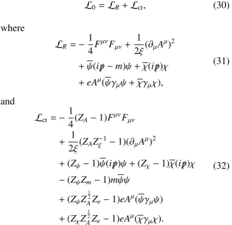
In order to renormalize QED, we consider the QED Lagrangian with Nf = 1+1 active flavor, one massive (muon) and one massless (electron) [50]:
L0=−
1 4F
µν 0 F0,µν+
1 2ξ0
(∂µAµ0)2 +ψ0(i/p−m0)ψ0+χ0(i/p)χ0 +e0Aµ0(ψ0γµψ0+χ0γµχ0).
(28)
In this approach, fields, couplings and masses are treated to bebare(denoted with the subscript 0). Bare quantities
amp@NNLO
FeynArts
FeynCalc AIDA
Reduze Kira
Amplitude to MIs
Analytical vs. Numerical
SecDec Analytical
MIs
Unrenormalized amplitude
Figure 2.Flowchart of the algorithm
are connected to therenormalizedones by
ψ0=Z
1 2
ψψ, χ0=Z
1 2
χχ, Aµ0=Z
1 2 AA
µ, ξ0=Zξξ, e0 =Zee, m0=Zmm.
(29)
The bare Lagrangian can be expressed in terms of the renormalized quantites:
L0 =LR+Lct, (30)
where
LR=−
1 4F
µνFµν+ 1
2ξ(∂µA
µ)2
+ψ(i/p−m)ψ+χ(i/p)χ +eAµ(ψγµψ+χγµχ),
(31)
and
Lct=−
1
4(ZA−1)F
µνFµν
+ 1 2ξ(ZAZ
−1
ξ −1)(∂µAµ)2
+(Zψ−1)ψ(i/p)ψ+(Zχ−1)χ(i/p)χ
−(ZψZm−1)mψψ
+(ZψZ
1 2
AZe−1)eAµ(ψγµψ) +(ZχZ
1 2
AZe−1)eA
µ(χγµχ).
(32)
Ward Identities in QED constrain ratios between the normalizationsZi[50].
ZA
Zξ =κξ, Z
1 2 A
ZξZe =
κe, (33)
whereκξandκeare arbitraryfiniteconstants. By choosing
κi=1, the normalizations become
Zξ=ZA, Ze=Z
−1 2
A . (34)
Note that the choice of the renormalization scheme for the photon field Aµ leads automatically to fix the same pre-scription to the couplinge. This is a direct consequence of the Ward Identities (34) in QED .
It is important to stress that Eq. (33) constrains only the divergent part of the normalizations, letting their finite part unconstrained. Hence, two different renormalization prescription forZeandZA can be chosen, e.g. ZA in
on-shellscheme andZein MS scheme. This alternative choice brings the Ward identity to be
Ze=Z
−1 2 A
finite=0, (35)
which yields no contradiction with Eq. (33).
Imposing the Ward identities (33), the counterterms Lagrangian becomes
Lct=−
1
4(ZA−1)F
µνFµν
+(Zψ−1)ψ(i/p)ψ+(Zχ−1)χ(i/p)χ
−(ZψZm−1)mψψ
+(Zψ−1)eAµ(ψγµψ) +(Zχ−1)eAµ(χγµχ).
(36)
Finally, by settingZi=1+δi
Lct=−
1 4δAF
µνFµν
+δψψ(i/p)ψ+δχχ(i/p)χ
−(δψ+δm+δψδm)mψψ
+δψeAµ(ψγµψ)+δχeAµ(χγµχ).
(37)
The Ward identities have been chosen in such a way that only field and mass renormalization is needed. The cou-pling constant eis automatically renormalized thanks to the Ward identities.
The counterterm Lagrangian provides additional Feyn-man rules, which lead to UV finite amplitude. Physical results can only be obtained by choosing a renormaliza-tion schemethat fixes the residual unphysical degrees of freedom.
Different renormalization schemes bring changes to the 4-point Green function. The S−matrix element
heµ|S|eµiis related to theamputated renormalizedGreen functionh0|T{ψ(p1)χ(p2)ψ(p3)χ(p4)} |0iamp=G4by
hµe|S|µei=(/p1−mP)/p2/p3(/p4−mP)G4, (38)
known as Lehmann-Symanzik-Zimmermann (LSZ) reduc-tion formula [51, 52]. The Dirac operators (/pi−mP) con-tain the wave-function corrections, andmPis thepole mass of the muon. Different renormalization scheme choices lead to different renormalized masses m, introducing a
residueat the pole massRψ ,1,
lim
/
p→mP
(/p−mP)
i /
p−m =Rψ
⇓
h0|T{ψ(p)ψ(−p)} |0i= iRψ
/ p−mP +
regular terms. (39)
The LSZ reduction formula changes according to the new residue, acquiring new factors [50]:
hµe|S|µei=(/p1−mP)/p2/p3(/p4−mP)
G4
RψRχ. (40)
Expressing the residue asRi=1+δRi, the order-by-order structure of the renormalized Green function become man-ifest
G4=Gtree+G1l+G2l+·,
δRi=δRi,1l+δRi,2l+· · ·,
(41)
which yields to the following structure
G4=Gtree
+[G1l−(δRψ,1l+δRχ,1l)Gtree] +[G2l−(δRψ,1l+δRχ,1l)G1l
−(δRψ,2l+δRχ,2l)Gtree+δRψ,1lδRχ,1lGtree]. (42)
The choice of theon-shellrenormalization scheme for the muon mass and fields setsδRψ,i=0 identically.
Therefore, the renormalization scheme choice applied in theµe→µescattering is:
- MS scheme for thecoupling, thephotonand theelectron
fields
- On-shell scheme for themuonfield and mass
The muon field is treated differently due to its non-vanishing mass. Despite of the complications it introduces at integration level, the opportunity to use on-shell scheme for the muon yields simplification at renormalization level.
8 Summary
There are 69 two-loop Feynman diagrams contributing to the QED NNLOµe-scattering process (Fig. 1). The com-plete amplitude gets contributions from ∼ 104 Feynman
integrals with maximum rank equal to 4.
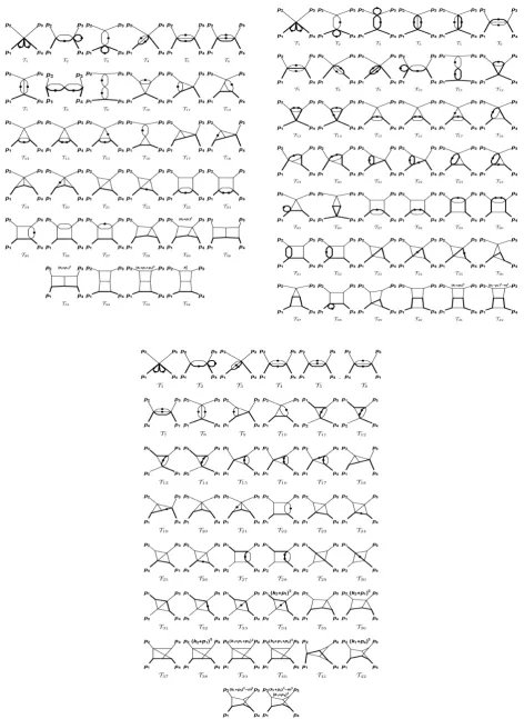
The differential equation method has allowed the an-alytical evaluation of the planar [18] and non-planar [19] sets of MIs. The consistency of the result has been checked by evaluating the MIs with GiNaC and comparing the re-sult with the numerical integration with SecDec, finding agreement between the two approaches.
At the present state of the calculation, the analyti-cal unrenormalized amplitude has been achieved. The renormalization strategy discussed in Section 7 is still in progress. A careful check of the cancellation of the UV divergencies is required in order to obtain a UV finite con-tribution.
The double-virtual contribution represents the most challenging part of the full µe-scattering cross section. However, the complete UV/IR finite NNLO amplitude can be achieved only by including all the contributions in Eq. (6). A particular care should be given to the soft and collinear limit due to photon emission from the electron, which in our approximation are treated as massless.
Real-virtual and double-real correction involve 1-loop and tree-level calculations, which can be dealt with the same technology shown in Section 6. For 1-loop am-plitudes, additional tools are available on the market e.g. GoSam[53] or Package-X [54].
9 Acknowledgment
This work has been supported by the Generalitat Valen-ciana, the Spanish Government and ERDF funds from the EU Commission and the Spanish Centro de Excelencia Severo Ochoa Programme (Grants No. SEJI/2017/019, FPA2017-84445-P and SEV-2014-0398).
References
[1] T. Blum, A. Denig, I. Logashenko, E. de Rafael, B.L. Roberts, T. Teubner, G. Venanzoni, The muon (g-2) theory value: Present and future(2013),1311.2198
[2] C. Carloni Calame, M. Passera, L. Trentadue, G. Ve-nanzoni, Physics Letters B746, 325–329 (2015) [3] G. Abbiendi, C.M.C. Calame, U. Marconi, C.
Mat-teuzzi, G. Montagna, O. Nicrosini, M. Passera, F. Piccinini, R. Tenchini, L. Trentadue et al., The Eu-ropean Physical Journal C77(2017)
[4] M. Alacevich, C.M. Carloni Calame, M. Chiesa, G. Montagna, O. Nicrosini, F. Piccinini, JHEP 02, 155 (2019),1811.06743
[5] M. Fael, JHEP02, 027 (2019),1808.08233
[6] M. Fael, M. Passera, Phys. Rev. Lett.122, 192001 (2019),1901.03106
[7] P. Mastrolia, T. Peraro, A. Primo, Journal of High Energy Physics2016(2016)
[8] P. Mastrolia, T. Peraro, A. Primo, W.J.T.
Bobadilla, Adaptive integrand decomposition
(2016),1607.05156
[9] A. Primo, Ph.D. thesis, Padua U. (2017) [10] W.J.T. Bobadilla, Ph.D. thesis, Padua U. (2017)
[11] K.G. Chetyrkin, F.V. Tkachov, Nucl. Phys. B192, 159 (1981)
[12] Laporta, International Journal of Modern Physics A
15, 5087 (2000)
[13] A. von Manteuffel, C. Studerus, Reduze 2 -distributed feynman integral reduction (2012),
1201.4330
[14] P. Maierhöfer, J. Usovitsch, P. Uwer, Comput. Phys. Commun.230, 99 (2018),1705.05610
[15] A.V. Kotikov, Phys. Lett.B254, 158 (1991)
[16] J.M. Henn, Journal of Physics A: Mathematical and Theoretical48, 153001 (2015)
[17] M. Argeri, S. Di Vita, P. Mastrolia, E. Mirabella, J. Schlenk, U. Schubert, L. Tancredi, JHEP03, 082 (2014),1401.2979
[18] P. Mastrolia, M. Passera, A. Primo, U. Schubert, Journal of High Energy Physics2017(2017) [19] S. Di Vita, S. Laporta, P. Mastrolia, A. Primo,
U. Schubert, Journal of High Energy Physics2018
(2018)
[20] G. HEINRICH, International Journal of Modern Physics A23, 1457–1486 (2008)
[21] G. Ossola, C.G. Papadopoulos, R. Pittau, Nuclear Physics B763, 147–169 (2007)
[22] P. Mastrolia, E. Mirabella, T. Peraro, Journal of High Energy Physics2012(2012)
[23] S. Badger, H. Frellesvig, Y. Zhang, Journal of High Energy Physics2012(2012)
[24] F. Tkachov, Physics Letters B100, 65 (1981) [25] G. Passarino, M.J.G. Veltman, Nucl. Phys. B160,
151 (1979)
[26] A.V. Smirnov, V.A. Smirnov, Journal of High Energy Physics2006, 001–001 (2006)
[27] W.L. van Neerven, J.A.M. Vermaseren, Phys. Lett.
137B, 241 (1984)
[28] P. Mastrolia, E. Mirabella, G. Ossola, T. Peraro, Physics Letters B718, 173–177 (2012)
[29] T. Hahn, Computer Physics Communications 140, 418 (2001)
[30] T. Peraro, JHEP07, 031 (2019),1905.08019
[31] A.G. GROZIN, International Journal of Modern Physics A26, 2807–2854 (2011)
[32] A.V. Smirnov, A.V. Petukhov, Lett. Math. Phys.97, 37 (2011),1004.4199
[33] J.M. Henn, Physical Review Letters110(2013) [34] R.N. Lee, Journal of High Energy Physics 2015
(2015)
[35] A. Smirnov, Journal of High Energy Physics2008, 107–107 (2008)
[36] A. Georgoudis, K.J. Larsen, Y. Zhang, Computer Physics Communications221, 203–215 (2017) [37] R.N. Lee, Journal of Physics: Conference Series523,
012059 (2014)
[38] W. Magnus, Commun. Pure Appl. Math. 7, 649 (1954)
[39] S. Blanes, F. Casas, J. Oteo, J. Ros, Physics Reports
[40] E. Remiddi, Nuovo Cim. A110, 1435 (1997),
hep-th/9711188
[41] M. ARGERI, P. MASTROLIA, International Journal of Modern Physics A22, 4375–4436 (2007)
[42] T. Gehrmann, E. Remiddi, Nuclear Physics B580, 485–518 (2000)
[43] S. Di Vita, P. Mastrolia, A. Primo, U. Schubert, Jour-nal of High Energy Physics2017(2017)
[44] S. Di Vita, T. Gehrmann, S. Laporta, P. Mastro-lia, A. Primo, U. Schubert, JHEP 06, 117 (2019),
1904.10964
[45] R. Bonciani, A. Ferroglia, T. Gehrmann, D. Maître, C. Studerus, Journal of High Energy Physics 2008, 129–129 (2008)
[46] R. Bonciani, A. Ferroglia, T. Gehrmann, C. Studerus, Journal of High Energy Physics 2009, 067–067 (2009)
[47] R. Bonciani, A. Ferroglia, T. Gehrmann, A. von Manteuffel, C. Studerus, Journal of High Energy
Physics2011(2011)
[48] S. Borowka, G. Heinrich, S. Jones, M. Kerner, J. Schlenk, T. Zirke, Computer Physics Communi-cations196, 470–491 (2015)
[49] T. Hahn, Computer Physics Communications 168, 78–95 (2005)
[50] M. Bohm, A. Denner, H. Joos, Gauge theories of the strong and electroweak interaction(2001), ISBN 9783519230458, 9783322801623, 9783322801609 [51] H. Lehmann, K. Symanzik, W. Zimmermann, Il
Nuovo Cimento (1955-1965)1, 205 (1955)
[52] M.D. Schwartz,Quantum Field Theory and the Stan-dard Model (Cambridge University Press, 2014), ISBN 1107034736, 9781107034730
[53] G. Cullen, N. Greiner, G. Heinrich, G. Luisoni, P. Mastrolia, G. Ossola, T. Reiter, F. Tramontano, The European Physical Journal C72, 1889 (2012) [54] H.H. Patel, Comput. Phys. Commun. 197, 276