A DISCRETE-TIME SLIDING MODE CONTROLLER
WITH MODIFIED FUNCTION FOR LINEAR
TIME-VARYING SYSTEMS
Deelendra Pratap Singh
1, Anil Sharma
2, Shalabh Agarwal
31,2
Department of Electronics & Communication Engineering, IET,
Mangalayatan University, Aligarh, Uttar Pradesh, (India)
Ocean Consultancy Services, Agra (India)
ABSTRACT
This paper contains the linear time varying systems with discrete time sliding mode control with modified switching
function. The changed sliding surface improves control input in the initial phase and reduces the chattering with
improved robustness. Also the system state is uniformly eventually bounded with better asymptotic convergence
under the existence of time varying disturbances.
Keywords: Discrete-Time Systems, Linear Time-Varying System, Sliding Mode Control
I
INTRODUCTION
chattering so the quasi sliding mode motion was developed which will not cross the sliding hyper plane in each step, but exists in a certain band around it. Then new reaching law technique control strategy is applied. Since the state is not crossing the sliding hyper plane consequently undesirable chattering is avoided. He guarantees convergence of the system state to a vicinity of predetermined fixed plane in finite time. In this way they achieve better regulation quality by reducing control effort [10]. Later on a discrete time sliding mode control was developed by Kang-Bak Park which works for linear time-varying systems. According to him the system state is globally uniformly ultimately bounded under the existence of the Time Varying Disturbance and uncertainties and asymptotically stable for the closed loop system. He set the magnitude of the ultimate bound to be very small simply by increasing the sampling frequency [12]. The above discrete time sliding mode control was also used practically in steering the Highway vehicles and in changing the lanes even in presence of the disturbance it found to be stable [13].Since the presence of uncertainties and disturbances in the discrete-time sliding mode control does not guarantee the invariant property and does not assure the asymptotic convergence of the system state. And at the initial level of reaching there is a lot of chattering occurs due to uncertain disturbances.
Thus in this paper a discrete time sliding mode controller with modified function for Linear Time-Varying Systems with different disturbances is proposed and verified by simulations that the new control is able to converge better than the previous control law. It guarantees that the system state is globally uniformly ultimately bounded under the existence of Time Varying disturbance and uncertainty and yields less chattering in the initial phase of the iterations. This paper can be organized as follows. Section II gives the problem formulation for the Linear Time Varying Systems. The deduction of the Reaching Law and Stability Analysis is carried out in Section III. Then the proposed algorithm is illustrated with Numerical Example followed by Simulation Results in Section IV. At last conclusion of comparison is discussed in Section V.
II
PROBLEM
FORMULATION
Let us consider a linear discrete time varying plant of the following form [12]:
x (k+1) = A(k)x(k) + Bu(k) + Dr(k) (1) where k=1,2,3...., x(·) ϵ Rn is the state vector, u(·) ϵ R is the scalar input. D(·) ϵ Rn
is the vector for external disturbance. A(·) ϵ Rn*n is the linear time varying system matrix. B ϵ Rn*1
is the input matrix. Let the sliding surface as:
S(k) = τ x (k) (2)
Where tT =Rnis assumed to be designed such that τ *B is non-singular.
For the system to be uniform asymptotically stable, the sliding dynamics can be represented as:
S (k) = 0 (3)
For the system (1) the sliding dynamics (3) can be written as:
For the above equation, the equivalent control input can be written as:
Ueq (k) = - ( τB) – 1[τA(k) x(k) + τD(k)] (5) Therefore for the above system, the dynamics in the sliding mode can be expressed as: X(k+1) = A(k) x(k) + B Ueq(k) + D(k)
= (I – B(τB) -1) [A(k) x(k) + D(k)] (6)
Thus we can say the C is assumed to be chosen such that the above sliding dynamics turns to be stable. A system is in a quasi-sliding mode when the dynamics of meets the following conditions [6].
1. Starting from any state, the moves towards the quasi-sliding surface defined by and crosses it in a finite period of time.
2. As the sliding surface is crossed by the first time the s(k) value changes around the surface in a zig-zag motion.
3. The sliding zig-zag motion is stable and stays inside a fixed band.
III DEFINITIONS [8]
1. The motion of a discrete-time system satisfying attributes (2) and (3) is called a quasi-sliding mode. The specified band which contains the quasi-sliding mode is called the quasi-sliding mode band is defined as:
{ x| - δ<S(k)< + δ} (7) Where 2δis the width of the band.
2. The quasi- sliding mode becomes an ideal quasi- sliding mode when.
3. A discrete time system is said to satisfy a reaching condition if the resulting system possesses all three conditions (1),(2) and (3).
The reaching law straightly dictates the dynamics of the switching function and for a discrete time system it can be stated as [8]:
S(k + 1) – S(k) = - qTs(k) – Tsgn(S(k)) (8) where ε > 0, q > 0, 1 – qT> 0, T > 0 is the sampling period.
IV
REACHING
LAW
AND
STABILITY
ANALYSIS
Let's begin with the incremental change of the switching mode i.e.:
S (k + 1) – S (k) = τ x (k + 1) - τ x(k) (9)
Substituting (1) into (9) gives:
S (k + 1) – S (k) = τA(k) x(k) + τBu(k) + τD(k) – τx(k) (10) Now comparing it to reaching law (8):
U(k) = - (τB)-1[τA(k) x(k) + τD(k) – τx(k) + qτTs(k) + ε Tsgn (τS(k)] (12) Substituting (12) into (1) gives the response of the linear discrete time linear Time varying plant.:
X(k + 1) = A(k) x(k) – B(τB)-1[τA(k) x(k) + τD(k) – τx(k) + qτTs(k) + ε Tsgn (τS(k)] + D(k) (13)
The sliding mode band is given by (7).The objective is to determine the bandwidth (2δ) so that when the trajectory moves into the band it remains stay within the band.
Multiply τ on both sides of (13) yield:
S(k + 1) = (1 – qT) S(k) – εTsgn(S(k)) (14)
where 1 – qT>0
In the above equation the sign of S (k + 1) must be opposite to that of S(k)& this reason is given by [3]: {x|s(x)| < ε T/1 – qT}
Therefore, the bandwidth is given by :
2δ = 2( ε T/1 – qT) (15)
In (15) the trajectory will more with a smaller band & with decreasing sampling period, the width of both the bands decreases.
In order to proof the system is in quasi-sliding mode, the reaching law can be established by mathematically proving:
S(k) [S(k + 1) – S(k)] < 0
S(k) .S(k + 1) – S2(k) < 0 (16)
Since,S(k) = 0 hence S2 is negligible and assumed to be zero. Therefore, :
S(k + 1).S(k) < 0 (17)
Now from (2) we can write (17) as: τ x(k + 1).τx(k) < 0
τ2 x(k)[(A(k) x(k) + D(k)) (1 – B(τB)-1τ] < 0 (18)
And for fulfilling the reaching law the values for matrices B and C should be chosen such that the productB(τB)-1τ must be greater than identity matrix I. And in our simulation it is shown thatA(k) B(τB)-1 is greater than A(k) hence obeying the condition for reaching law.
V
SIMULATION
RESULTS
Consider the following Discrete-Time Varying System matrices [16]:
Example 1:
, ,,
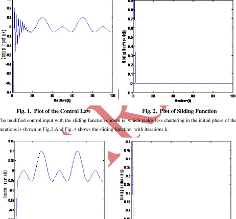
The sliding surface chosen is which is same as proposed in [12].For initial condition x(0) = [0.5 0.5] the SMC input is derived and the simulation results are shown in Fig. 1 and 2.Fig.1 shows the control input which is similar as proposed by Kang-Bak Park.
Fig. 1. Plot of the Control Law
Fig. 2. Plot of Sliding Function
The modified control input with the sliding function chosen is which yields less chattering in the initial phase of the iterations is shown in Fig.3.And Fig. 4 shows the sliding function with iterations k.
Example 2:
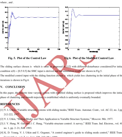
, ,, where , and .
Fig. 5. Plot of the Control Law Fig 6. Plot of the Modified Control Law
.The sliding surface chosen is which is same as proposed in [12] with different disturbance considered.For initial condition x(0) = [0.5 0.5] the SMC input is derived and the simulation results are shown in Fig.5.
The modified control input with the sliding function chosen is which yields less chattering in the initial phase of the iterations is shown in Fig.6.
V.
CONCLUSION
In this paper, the discrete time varying system with modified sliding surface is proposed which improves the initial phase of chattering and smooth trajectory is established which is uniformly eventually bounded.
REFERENCES
[1] V. I. Utkin, “Variable structure systems with sliding modes,”IEEE Trans. Automat. Contr., vol. AC-22, no. 2.pp. 212-222, 1977.
[2] V. I. Utkin, “Sliding Modes and Their Application to Variable Structure Systems,” Moscow: Mir. 1977.
[3] J. Y. Hung, W. Gao and J. C. Hung, “Variable structure control: A survey,” IEEE Trans. Ind. Electron., vol. 40, no. 1, pp. 2–21, Feb. 1993.
[4] K. D. Young, V. I. Utkin and U. Ozguner, “A control engineer’s guide to sliding mode control,” IEEE Trans. Control Syst., vol. 7, no. 3,pp. 328–342, May 1999.
[7] A. Bartolini, A. Ferrara, and V. Utkin, “Adaptive mode control in discrete-time systems,” Automatica, vol. 31, no. 5, pp. 769–773, 1995.
[8] W. Gao, Y. Wang and A. Homaifa, “Discrete time variable structure control systems,” IEEE Trans. Ind. Electron., vol. 42, pp. 117–122, Apr.1995.
[9] C.Y.Chan, “Discrete Adaptive Sliding-mode Tracking Controller,” Automatica, vol. 33, no. 5, pp. 999–1002, 1997.
[10] AndrzejBartoszewicz, “Discrete-Time Quasi-Sliding-Mode Control Strategies,” IEEE Trans. Industrial. Electronics, vol. 45,No.4 Aug. 1998.
[11] David Munoz et.al, "An Adaptive Sliding-Mode Controller for Discrete Nonlinear Systems," IEEE Trans. Industrial. Electronics, vol. 47,No.3 Jun.
2000.
[12] Kang-BakPark,”Discrete-Time Sliding Mode Controller for Linear Time-Varying Systems with Disturbances,” ICASE, Korea, Vol 2,No.4,Dec.2000.
[13] J.Kharaajoo, "Discrete-time sliding mode control design for linear time-varying systems: application to steering control of highway vehicles," Mechatronics, ICM-04. Proceedings of the IEEE International Conference on, On page(s): 113 - 116, 2004.
[14] O. Kaynak and A. Denker, “Discrete-time sliding mode control in presence of system uncertainty,” Int. J. Contr., vol. 57, no. 5, pp. 1177–1189, 1993.
[15] D. Muñoz, “Discrete sliding mode controller for nonlinear systems,” M.S. thesis (in Spanish), Dep. Elect. Eng., Faculty Eng., Univ. Concepción, Concepción, Chile, 1997.