Thermophysical properties of 22 pure metals in the solid and liquid state

(1)

– The pulse-heating data collection

T. Hüpf1, C. Cagran1, and G. Pottlacher1

1

Graz University of Technology, Institute of Experimental Physics, 8010 Graz, Austria

Abstract.The workgroup of subsecond thermophysics in Graz has a long tradition in performing fast pulse-heating experiments on metals and alloys. Thereby, wire-shaped specimens are rapidly heated (108_{K/s) by a} large current-pulse (104 A). This method provides thermophysical properties like volume-expansion, enthalpy and electrical resistivity up to the end of the liquid phase. Today, no more experiments on pure metals are to be expected, because almost all elements, which are suitable for pulse-heating so far, have been investigated. The requirements for pulse-heating are: a melting point which is high enough to enable pyrometric temperature measurements and the availability of wire-shaped specimens. These elements are: Co, Cu, Au, Hf, In, Ir, Fe, Pb, Mo, Ni, Nb, Pd, Pt, Re, Rh, Ag, Ta, Ti, W, V, Zn, and Zr. Hence, it is the correct time to present the results in a collected form. We provide data for the above mentioned quantities together with basic information on each material. The uniqueness of this compilation is the high temperature range covered and the homogeneity of the measurement conditions (the same method, the same laboratory, etc.). The latter makes it a good starting point for comparative analyses (e.g. a comparison of all 22 enthalpy traces is in first approximation conform with the rule of Dulong-Petit which states heat capacity – the slope of enthalpy traces – as a function of the number of atoms). The data is useful for input parameters in numerical simulations and it is a major purpose of our ongoing research to provide data for simulations of casting processes for the metal working industry. This work demonstrates some examples of how a data compilation like this can be utilized. Additionally, the latest completive measurement results on Ag, Ni, Ti, and Zr are described.

1 Fast pulse-heating

1.1 Experimental

In the technique of fast pulse-heating electrically conducting samples are heated rapidly by the passage of a large current pulse (approx. 10000 A). The energy is stored in a capacitor which is then discharged over the sample. The resistive heating continues up to the transition to the gas phase. Due to the high heating rate (108 K/s) the specimen maintains its position even in the liquid phase. This is the key-feature of pulse-heating. The experimental duration is typically 50 µs; consequently, heat-loss and chemical reactions are strongly inhibited.

During heating, several quantities are measured simultaneously: The temperature T is measured by means of pyrometry. The voltage drop along the specimen is measured by two knife-edge contacts directly touching the surface of the sample. The current I is measured with an induction coil. The thermal expansion is measured with a fast CCD-camera. From these recorded pictures the diameter D can be evaluated in steps of 5 µs or 2.5 µs. From the raw data, enthalpy H, resistivity at initial geometry IG, and radial expansion D2/D02 can be

calculated as a function of temperature (D0: diameter at room temperature). Specific resistivity  is obtained by multiplying IG with D2/D02. Due to the clamping the fraction D2/D02 is equal to the volumetric expansion V/V0 (V: volume, V0: volume at room temperature), because the axial component of expansion is deflected in radial direction.

For more details about the experimental setup see [1].

1.2 The situation of today

There are certain requirements concerning the specimens: They must be electrically conducting, the meltingpoint has to be high enough to enable pyrometric temperature measurement, and specimens must be available in the shape of a wire. The latter restriction creates a technological challenge. Some elements, which are too brittle to be drawn as a wire, can be cut into rectangular wires by electro-erosion machining. These wires can be processes by pulse-heating as well, except for the expansion measurement.

Today almost all elements which fulfill the requirements have been investigated at the laboratory in Graz. These elements are: Co, Cu, Au, Hf, In, Ir, Fe, Pb, © Owned by the authors, published by EDP Sciences, 2011

(2)

Mo, Ni, Nb, Pd, Pt, Re, Rh, Ag, Ta, Ti, W, V, Zn, and Zr (ordered alphabetically by spoken names). The measurements are published in various different journals by different authors, which are – or have been – members of the ‘Workgroup of Subsecond Thermophysics’ at the TU Graz.

Ongoing research is mainly dedicated to binary alloys [2] and alloys with industrial relevance.

2 Creation of a compilation

To summarize all measurements on pure elements and to provide easy access, it was decided to make a compilation. Usually, such data compilations try to assemble such kinds of information about an element, which are appropriate for the user. Hence, different measurement techniques and different workgroups are combined to obtain the best result. In the case of the pulse-heating data collection the situation is different. The measurement technique and the laboratory are identical for every element. This is the central theme of the compilation. On the one hand the homogeneity of results, which is a good starting point for comparative analyses, and on the other hand the large temperature range that can be covered with pulse-heating, make this compilation an exceptional data collection.

2.1. Quantities

It is common to start any investigation with a basic survey. This was implemented in the compilation by including a bachelor-thesis, which is a conglomeration of easy available basic information. Amongst other things the topics ‘history’, ‘common uses’, and ‘relevance in life’ are covered in this thesis in an easy going way, e. g. by text, referring to internet pages.

The stated quantities obtained by pulse-heating are thermal expansion (D2/D02), enthalpy (H), resistivity with initial geometry (IG), and resistivity () as a function of temperature. They are displayed graphically and by polynomials, as well. Specific heat capacity cp and heat of

fusion H are calculated from the enthalpy polynomials. Thermal conductivity  and thermal diffusivity a can easily be calculated by equations (1) and (2):

 = L T-1 (1)

a(T) = L T cp-1IG(T)-1 d0-1 (2)

L is the Lorentz-number (2.45·10-8 V2K-2), d0 is the density at room temperature.

2.2 Completive measurements

To complete the measurement results it was necessary to perform new measurements. The thermal expansion of Ag, Ni, Ti, and Zr belongs to these follow-up measurements.

As  has to be calculated from IG combined with thermal expansion, new measurements of thermal expansion can be considered to obtain ‘better’ values for

 which prior to that had to be combined with expansion values from the literature.

2.2.1 Silver

The measurements on silver are published in [3]. Follow-up measurements of thermal expansion for the liquid phase (1234 K < T < 2000 K) yield (3):

D2(T)/D02 = 1.002 + 4.736·10-5T (3)

Including these values in the calculation of  leads to (1234 K < T < 1950 K) (4):

(T) = 4.592·10-2 + 9.856·10-5T (4)

 is given in µ m. The resistivity at the onset of melting is s = 0.090 µm (subindex s: solid), the resistivity at the end of melting is l = 0.168 µ m (subindex l: liquid). This lead to an increase of resistivity at melting of  = 0.078 µ m.

2.2.2 Nickel

The measurements on nickel are published in [4]. Follow-up measurements of thermal expansion for the solid phase (300 K < T < 1728 K) yield (5):

D2(T)/D02 = 1.000 – 6.604·10-6T + 2.738·10-8T2 (5)

And for the liquid phase (1728 K < T < 2600 K) (6):

D2(T)/D02 = 0.930 + 9.730·10-5T (6)

(T) = -3.734·10-2 + 1.857·10-4T + 5.411·10-7T2 (7)

In the range 627 K < T < 1270 K (8):

(T) = -0.181 + 0.118·10-2T – 8.145·10-7T2

+ 2.406·10-10T3 (8)

In the range 1300 K < T < 1715 K (9)

(T) = 0.106 + 3.456·10-4T – 2.920·10-8T2 (9)

(T) = 0.667 + 1.043·10-4T (10)

 is given in µ m. The resistivity at the onset of melting is s = 0.616 µ m, the resistivity at the end of melting is l = 0.848 µ m. This lead to an increase of resistivity at melting of  = 0.232 µ m.

2.2.3 Titanium

(3)

D2(T)/D02 = 0.938 + 6.108·10-5T (11)

(T) = 1.7063 + 1.483·10-5T (12)

 is given in µ m. The resistivity at the end of melting is l = 1.735 µ m.

2.2.4 Zirconium

The measurements on zirconium are published in [6]. Follow-up measurements of thermal expansion for the solid phase (1500 K < T < 2127 K) yield (13):

D2(T)/D02 = 0.984 + 2.861·10-6T (13)

D2(T)/D02 = 0.920 + 5.944·10-5T (14)

(T) = 0.830 + 2.592·10-4T (15)

(T) = 1.258 + 8.735·10-5T (16)

 is given in µ m. The resistivity at the onset of melting is s = 1.378 µ m, the resistivity at the end of melting is l = 1.446 µ m. This lead to an increase of resistivity at melting of  = 0.068 µ m.

3 Comparative Analyses

3.1 Enthalpy H

Having summarized data is always a motivation for doing comparative analyses. In a first try, one can plot everything into one graph. Figure 1 shows the enthalpy traces of 19 elements as a function of temperature.

Of course, such an illustration is not the best way to present results for every purpose due to difficulties with labeling, but nevertheless, this graph exhibits information about the enthalpy. We can easily identify three bundles of traces, which are correlated to the position of the respective element in the periodic system of the elements (4th, 5th, and 6th period).

1000 2000 3000 4000 5000 0

500 1000 1500 2000

E

n

thalp

y /

kJ

kg

-1

Temperature / K

Fig. 1. Enthalpy traces of 19 elements as a function of temperature.

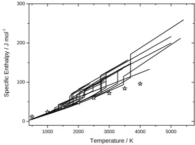
If the same enthalpy traces are plotted in molar units (J·mol-1), their relative positions in the graph change remarkably (see figure 2).

1000 2000 3000 4000 5000 0

100 200 300

S

p

e

c

if

ic

En

th

alp

y

/

J

m

o

l

-1

Temperature / K

Fig. 2. Enthalpy traces of 19 elements in molar units. Stars: calculation according to equation (18).

The three bundles have contracted into one. This is some kind of experimental indication that the enthalpy mainly depends on the number of atoms. It is consistent with the rule of Dulong-Petit (17):

c = 3 N k (17)

The heat capacity c, which is the slope of the enthalpy traces, depends on the number of atoms N and the Boltzmann-constant k. The calculation for one mole (NA) yields (18) [7]:

cmol = 3 NA k = 24.9 J·mol-1·K-1 (18)

The enthalpy calculation thereof yields the stars in figure 2.

3.2 Heat of fusion H

The same approach can be applied to the heat of fusion

(4)

the respective position of the melting point (x-axis: temperature of melting point, y-axis: heat of fusion). No particular trend can be read out of this graph.

1500 2000 2500 3000 3500 100

200 300 400



H /

kJ·kg

-1

Temperature / K

W

Ag

Au

V

Rh

Re Ta Mo

Nb

Ir Ni

Hf Pt

Zr Cu

Co

Pd Fe Ti

Fig. 3. Heat of fusion as a function of the respective melting-point.

This time we convert the graph by changing the abscissa to enthalpy at melting in the solid Hs instead of temperature. The result can be seen in figure 4.

200 400 600 800 1000 1200 100

200 300 400



H /

kJ·kg

-1

H_s / kJ·kg-1

Au

Ti Fe Mo

Nb

W

Co Ni

Rh

Zr Cu

Ir

Ta

Re Pd

Hf Pt Ag

V

Fig. 4. Heat of fusion as a function of enthalpy at melting in the solid phase Hs. Dashed line: visualization of increasing trend.

In the new graph an increasing trend is recognizable (dashed line). Elements which need more energy input to reach the melting-temperature also need more energy input to be molten.

3.3 Resistivity 

To draw all electrical resistivity traces into one graph leads to the result in figure 5.

The traces in figure 5 are hard to compare. Pulse-heating results always cover the temperature-region around the melting-temperature. Only by extrapolation one could make a section at a fixed temperature to compare all resistivities.

1000 2000 3000 4000 5000 0.5

1.0 1.5

El

ect

rical resist

ivit

y /

µ



·m

Temperature / K Ag

Cu

Au Pt

Hf

Fig. 5. Electrical resistivity of 19 elements as a function of temperature.

3.4 Expansion

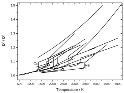
All traces of expansion were drawn into one graph to obtain figure 6.

500 1000 1500 2000 2500 3000 3500 4000 4500 5000 1.0

1.1 1.2 1.3 1.4 1.5

D

2 /

D

2 0

Temperature / K Re Cu

Fig. 6. Relative expansion as a function of temperature. Rectangles: expansion at the onset of melting.

At room temperature the factor of expansion equals unity for every element. Where available, the expansion at the onset of melting is displayed in figure 6. The average value of expansion until melting for these twelve elements is 6.3%.

If this was a general behavior, one would have to conclude, that the expansion coefficient of high melting metals was always low by trend.

3.5 Thermal conductivity and thermal diffusivity

(5)

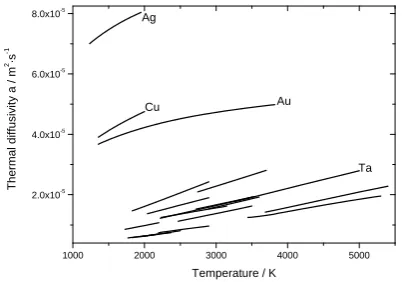
to equation (2), which includes room temperature density and heat capacity as well. The traces for the liquid phase are displayed in figure 7.

1000 2000 3000 4000 5000 2.0x10-5

4.0x10-5

6.0x10-5

8.0x10-5

Ther

mal diffusiv

ity

a

/ m

2·s

-1

Temperature / K Ag

Cu Au

Ta

Fig. 7. Thermal diffusivity of 19 elements as a function of temperature.

The interaction of , cp, and density leads to the

difference in distribution between figure 5 and figure 7: Silver has by far the highest thermal diffusivity. Copper and gold are in between silver and the rest of the elements. All other investigated metals are quite similar in their thermal diffusivity.

4

Summary

The ‘Workgroup of Subsecond Thermophysics’ in Graz has performed a lot of measurements on pure metals using the method of fast pulse-heating. As the focus of ongoing research is no longer on pure elements, but on alloys instead, it was decided to make a compilation of finished measurements. New measurements were performed to complete the data.

The follow up measurements on silver, nickel, titanium, and zirconium are presented in section ‘Completive measurements’. New results of thermal expansion give new values for electrical resistivity, which up to this time had to include expansion values from the literature.

We consider this data-collection as a good starting-point for comparative analyses. In this context the unusual – or even unaesthetic – procedure to draw all elements into one graph, seems justified. Some examples are given in section 3: The appearance of the enthalpy traces depends dramatically on the used set of units (compare figure 1 and 2). The heat of fusion is once plotted against melting-temperature (figure 3) and once plotted against enthalpy at melting in the solid (figure 4). All resistivity curves are shown in figure 5. From the thermal expansion traces (figure 6) the average of thermal expansion at the onset of melting was calculated, yielding 6.3%. The behavior of derived quantities like thermal diffusivity depends on the interaction of the input quantities. Consequently, the distribution of thermal diffusivity curves (figure 7) is quite different from the inverse distribution of resistivity curves.

Although for us this data-collection is a summary and somehow the closure of our pure-elements-research, we hope that it will also act as a starting-point for new discussions and collaborations with experimentalists and theoreticians as well.

About the availability of the compilation please contact Prof. Dr. Gernot Pottlacher ([email protected]).

Acknowledgement

The project Electrical Resistivity Measurement of High Temperature Metallic Melts is sponsored by the Austrian Space Applications Programme (ASAP) of the FFG, Sensengasse 1, 1090 Wien.

References

1. T. Hüpf, C. Cagran, B. Wilthan, G. Pottlacher, J. Phys.: Condens Matter 21 (2009)

2. T. Hüpf, C. Cagran, E. Kaschnitz, G. Pottlacher, Thermochimica Acta, 494 (2009)

3. C. Cagran, B. Wilthan, G. Pottlacher,

Thermochimica Acta, 445 (2006)

4. B. Wilthan, C. Cagran, G. Pottlacher, Int. J. Thermophys. 25 (2004)

5. B. Wilthan, C. Cagran, G. Pottlacher, Int. J. Thermophys. 26 (2005)

6. C. Brunner, C. Cagran, A. Seifter, G. Pottlacher,

Temperature: Its measurement and control in science and industry, volume 7 (American Institute of Physics, 2003)