IJCSMC, Vol. 8, Issue. 9, September 2019, pg.167 – 171 The Examination of Analyzing Data by Algorithm Performance

Available Online at www.ijcsmc.com

International Journal of Computer Science and Mobile Computing

A Monthly Journal of Computer Science and Information Technology

ISSN 2320–088X

IJCSMC, Vol. 8, Issue. 9, September 2019, pg.167 – 171

The Examination of Analyzing Data by

Algorithm Performance

Farhad Shamssoolari

Unit E4- Morvarid residential complex- Jouybar DE.(Dead End) - Shad Street- Mollasadra Street- Vanak Sq.-Tehran- Iran. Postal Code: 1435793885

Email:[email protected] Phone Number: +989129751845

Abstracts: An algorithm is a specified set of rules/instructions that the computer will follow to solve a particular

problem. In other words, we need to tell the computer how to process the data, so we can make sense of it. Data

analysis has many facets, ranging from statistics to engineering. In this paper basic models and algorithms for

data analysis are discussed [Songyi Xiao, Wenjun Wang, Hui Wang,2019]. Novel uses of cluster analysis,

precedence analysis, and data mining methods are emphasized. The software for the cluster analysis algorithm

and the triangularization is presented. The efficiency or complexity of the algorithm is nothing but the number of

steps executed by the algorithm to achieve the results. In theoretical analysis of algorithms, it is common to

estimate their complexity in asymptotic sense, i.e., to estimate the complexity function for reasonably large length

of input. It's also easier to predict bounds for the algorithm than it is to predict an exact speed. Asymptotic

notation is a shorthand way to write down and talk about 'fastest possible' and 'slowest possible' running times

for an algorithm, using high and low bounds on speed. Big O notation, omega notation and theta notation are

used to this end [Dr.N.Sairam & Dr.R.Seethalakshmi , 2010].

Keywords: Algorithm, Data, Performance, Analysing Data

1. Introduction:

Like other bio-inspired algorithms, ABC is also a population-based stochastic method. Bees in the population try to find new food sources (candidate solutions). According to the species of bees ,ABC consists of three types of bees: employed bees, onlooker bees, and scouts. The employed bees search the neighbourhood of solutions in the current population, and they share their search experiences with the onlooker bees. Then, the onlooker bees choose better solutions and re-search their neighbourhoods to find new candidate solutions. When solutions cannot be improved during the search, the scouts randomly initialize them[Karaboga, D.; Akay, B.2009].

line that stays within bounds. Asymptotic notation is a shorthand way to write down and talk about 'fastest possible' and 'slowest possible' running times for an algorithm, using high and low bounds on speed. Big O notation, omega notation and theta notation are used to this end[Dr.N.Sairam & Dr.R.Seethalakshmi , 2010].

To learn an algorithm well, one must implement it. Accordingly, the best strategy for understanding the programs presented in this book is to implement and test them, experiment with variants, and try them out on real problems. We will use the Pascal programming language to discuss and implement most of the algorithms; since, however, we use a relatively small subset of the language, our programs are easily translatable to most modern programming languages. Readers of this book are expected to have at least a year’s experience in programming in high- and low-level languages. Also, they should have some familiarity with elementary algorithms on simple data structures such as arrays, stacks, queues, and trees. (We’ll review some of this material but within the context of their use to solve particular problems.) Some elementary acquaintance with machine organization and computer architecture is also assumed. A few of the applications areas that we’ll deal with will require knowledge of elementary calculus. We’ll also be using some very basic material involving linear algebra, geometry, and discrete mathematics, but previous knowledge of these topics is not necessary.[ Hoare, C. A. R. “Quicksort, 1998]

To begin, we’ll consider a Pascal program which is essentially a translation of the definition of the concept of the greatest common divisor into a programming language.[ Songyi Xiao, Wenjun Wang, Hui Wang, Dekun Tan, Yun Wang , 2019]

The body of the program above is trivial: it reads two numbers from the input, then writes them and their greatest common divisor on the output.

The GCD function implements a “brute-force” method: start at the smaller of the two inputs and test every integer (decreasing by one until 1 is reached) until an integer is found that divides both of the inputs. The built-in function ABS is used to ensure that GCD is called with positive arguments. (The mod function is used to test whether two numbers divide: U mod V is the remainder when U is divided by V, so a result of 0 indicates that v divides U.) .[ Songyi Xiao, Wenjun Wang, Hui Wang, Dekun Tan, Yun Wang , 2019]

Many other similar examples are given in the Pascal User Manual and Report. The reader is encouraged to scan the manual, implement and test some simple programs and then read the manual carefully to become reason-ably comfortable with most of the features of Pascal.[ Jeffrey J. McConnell Canisius College,2015.]

2.Methods

2.1.Research Context

The research took place in Tehran, a poor municipality in northern Karaj. The areas chosen to carry out the research were Tehran National Library, which has been the most popular resource of studying, with lots of books, articles, thesis and disertations. Collection of those references have helped me to gather much information which I have needed. Primary researching has also assisted me to find useful and practical topics to usage them in this article.

2.2. Participants

First of all, we ought to test how algorithm carries out. Time taken by an algorithm? performance measurement or Apostoriori Analysis: Implementing the algorithm in a machine and then calculating the time taken by the system to execute the program successfully. Performance Evaluation or Apriori Analysis.[ Hoare, C. A. R.1998] Before implementing the algorithm in a system. This is done as follows. How long the algorithm takes :-will be represented as a function of the size of the input. f(n)→how long it takes if ‘n’ is the size of input. How fast the function that characterizes the running time grows with the input size. “Rate of growth of running time”. The algorithm with less rate of growth of running time is considered better.

2.3. Measures

How algorithm is a technology?

We discuss approximation algorithms for optimization problems.[ Hochbaum, D.1997] An optimization problem consists in finding the best (cheapest, heaviest, etc.) element in a large set P , called the feasible region and usually specified implicitly, where the quality of elements of the set are evaluated using a function f (x), the objective function, usually something fairly simple. The element that minimizes (or maximizes) this function is said to be an optimal solution of the objective function at this element is the optimal value.

optimal value = min{f (x) | x

∈

P} (1)

per second, so that computer A is1000 times faster than computer B in raw computing power. To make the difference even more dramatic, suppose that the world’s craftiest programmer codes in machine language for computer A, and the resulting code requires instructions to sort n numbers. Suppose further that just an average programmer writes for computer B, using a high-level language with an inefficient compiler, with the resulting code taking 50n LG n instructions. .[ Yanjiao Wang and Tianlin Du,2019]

Computer A (Faster) Computer B(Slower)

Running [Bellman, R. and Dreyfus 2007]time grows like2n.Grows inn logn.10 billion instructions per sec. 10 million instruction per sec 2n.

2.4. Procedure

Before going for growth of functions and asymptotic notation let us see how to analyses an algorithm.

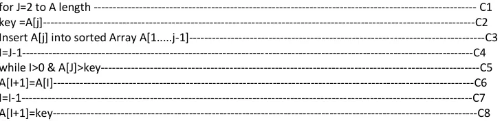
How to analyse an Algorithm. Let us form an algorithm for Insertion sort (which sort a sequence of numbers).The pseudo code for the algorithm is give below.

Pseudo code:

for J=2 to A length --- C1 key =A[j]---C2 Insert A[j] into sorted Array A[1...j-1]---C3 I=J-1---C4 while I>0 & A[J]>key---C5 A[I+1]=A[I]---C6 I=I-1---C7 A[I+1]=key---C8

Main Debate

1. Performance Analysis

An Algorithm is a step by step procedure to achieve a required result and an algorithm is a sequence of computational steps that transform the input into the output.[ Bentley, J., Johnson, D., Leighton, F, 2017]

1.1 An approximation algorithm for minimum-degree spanning tree

Nonetheless, the minimum-degree spanning-tree problem has a remarkably good approximation algorithm [Hochbaum, D. S.,2019]. For an input graph with m edges and n vertices, the algorithm requires time slightly more than the product of m and n. The output is a spanning tree whose figures in this part.[ Hoare, C. A. R.1998]

Figure 1: On the left is an example input graph G. On the right is a spanning tree T that might be found by the approximation algorithm. The shaded circle indicates the nodes in the witness set S.

Figure 2: The figure on the left shows the r trees T1, . . . , Tr obtained from T by deleting the nodes of S. Each tree is indicated by a shaded region. The figure on the right shows that no edges of the input graph G connect different trees Ti.[Hochbaum, D.1997] degree is guaranteed to be at most one more than the minimum degree. For example, if the graph has a Hamiltonian path, the output is either such a path or a spanning tree of degree three. Given a graph G, the algorithm naturally finds the desired spanning tree T of G. The algorithm also finds a witness — in this case, a set S of vertices proving that T ’s degree is nearly optimal. .[Hochbaum, D.1997]

Namely, let k denote the degree of T , and let T1, T2, . . . , Tr be the subtrees that would result from T if the vertices of S were deleted. The following two properties are enough to show that T ’s degree is nearly optimal.

1. There are no edges of the graph G between distinct trees TI, and

2. the number r of trees TI is at least |S|(k − 1) − 2(|S| − 1)

Figure 3: The figure on the left shows an arbitrary spanning tree T* for the same input graph G. The figure on the right has r shaded regions, one for each subset VI of nodes corresponding to a tree TI in Figure 3.2. The proof of the algorithm’s performance guarantee is based on the observation that at least r + |S| − 1 edges are needed to connect up the Vi’s and the nodes in S.

Hence we obtain

1.1 Asymptotic Analysis

The efficiency or complexity of the algorithm is nothing but the number of steps executed by the algorithm to achieve the results. In theoretical analysis of algorithms, it is common to estimate their complexity in asymptotic sense, i.e., to estimate the complexity function for reasonably large length of input[ Dr. M.R. Kabat – Module II [Dr. R. Mohanty – Module III 2012.]. It's also easier to predict bounds for the algorithm than it is to predict an exact speed. That is, "at the very fastest ,this will be slower than this" and "at the very slowest, this will be at least as fast as this" are much easier statements to make than "this will run exactly at this speed". Asymptotic means a line that tends to converge to a curve, which may or may not eventually touch the curve. It's a line that stays within bounds[Lawler, E., Lenstra, J., Kan, A , 2013]. Asymptotic notation is a shorthand way to write down and talk about 'fastest possible' and 'slowest possible' running times for an algorithm, using high and low bounds on speed. Big O notation, omega notation and theta notation are used to this end.[ Dr. M.R. Kabat – Module II Dr. R. Mohanty – Module III 2012.]

1.2.1 Big O notation

Big O notation is a mathematical notation used to describe the asymptotic behaviour of functions. Its purpose is to characterize a function's behaviour for large inputs in a simple but rigorous way that enables comparison to other functions. More precisely, it is used to describe an asymptotic upper bound for the magnitude of a function in terms function. It is the formal method of expressing the upper bound of an algorithm's running time. It's a measure of the longest amount of time it could possibly take for the algorithm to complete.[ Bellman, R. and Dreyfus, S,2017]

1.2.1.1 Definition

The function F(N) = O(G(N)) (read as “F of n is big oh of G of N”) if(read as “if and only if”) there NPTEL – Computer Science & Engineering – Parallel Algorithms Joint Initiative of IITs and IISC – Funded by MHRD Page 8 and 9 exist positive constants C and N0 such that F(N)<= C.G(N) for all N, N>=N0.[ Yanjiao Wang and Tianlin Du,2019]

Using O notation, we can often describe the running time of an algorithm merely by inspecting the algorithm’s overall structure. Moreover, it is important to understand that the actual running time depends on the particular input of size n. That is, the running time is not really a function of n. What we mean when we say “the running time is O(n2)” is that the worst-case running time (which is the function of n) is O(n2), or equivalently, no matter what particular input of size n is chosen for each value of n, the running time on that set of inputs is O(n2).[ Karaboga, D.; Akay, B. A , 2009]

1.2.2 Theta Notation

The theta notation is used when the function F can be bounded both from above and below by the same function G.

1.2 Performance Metrics for Parallel Systems

Taking the minimization problem as an example, SSA requires that there is only one squirrel at each tree, assuming the total number of the squirrels is N, therefore, there are N trees in the forest.[Mr. S.K. Sathua , 2012

]

All the N trees contain one hickory tree and Nfs (1 < Nfs< N) acorn trees; the others are normal trees which have no food. The hickory tree is the best food resource for the squirrels and the acorn tree takes second place. Nfs can be different depending on the different problems. Ranking the fitness values of the population in ascending order, the squirrels are divided into three types: individuals located at hickory trees (Fh), individuals located at acorn trees (Fa) and individuals located at normal trees (Fn).

Fh refers to the individual with the minimum fitness value, Fa contains the individuals whose fitness rank 2 to Nfs + 1 and the

remaining individuals are noted as Fn. In order to find the better food resource, the destination of Fa is Fh; the destinations of FN

Acknowledgements

I would like to express my special thanks of gratitude to my father and my mother and all people who have helped me.

Results

This paper proposes an improved squirrel search algorithm. In terms of SSA, the winter searching method cannot develop the search space sufficiently, and the summer searching method is too random to guarantee the convergence speed. ISSA introduces the jumping search method and the progressive search method. For the jumping search method, the ‘escape’ operation in winter supplements the population diversity and fully exploits the search space, while the ‘death’ operation in summer explores the search space more sufficiently and improves the convergence speed. Aside from this, the mutation in the progressive search method retains the evolutionary information more effectively and maintains the population diversity. ISSA selects the suitable method by the linear regression selection strategy according to the variation tendency of the best fitness value, which improves the robustness of the algorithm. Compared with SSA, ISSA pays more attention to developing the search space in winter, and pays more attention to exploring around the elite individual in summer, which keeps a good balance between development and exploration improves the convergence speed and the convergence accuracy. Moreover, ISSA selects a proper search strategy along with the optimization processing, so ISSA has greater possibilities in finding the optimal solution. The experimental results on 21 benchmark functions and the statistical tests show that the proposed algorithm can promote the convergence speed, improve the convergence accuracy and maintain the population diversity at the same time .Furthermore, ISSA has obvious advantages in convergence performances compared with other five intelligent evolutionary algorithms.

References:

1. Songyi Xiao, Wenjun Wang, Hui Wang, Dekun Tan, Yun Wang, Xiang Yu and Runxiu Wu , An Improved Artificial Bee Colony Algorithm Based on Elite Strategy and Dimension Learning , 2019

2. Dr.N.Sairam & Dr.R.Seethalakshmi School of Computing, SASTRA Univeristy, Thanjavur-613401.2010

3. LECTURE NOTES ON DESIGN AND ANALYSIS OF ALGORITHMS B. Tech. 6thSemester Computer Science & Engineering and Information Technology Prepared by Mr. S.K. Sathua – Module I Dr. M.R. Kabat – Module II Dr. R. Mohanty – Module III 2012.

4. Analysis of Algorithms: An Active Learning Approach Jeffrey J. McConnell Canisius College,2015.

5. Yanjiao Wang and Tianlin Du , An Improved Squirrel Search Algorithm for Global Function Optimization , 2019 6. Bellman, R. and Dreyfus, S. Applied Dynamic Programming. Princeton University Press, Princeton, NJ, 2017

7. Bentley, J., Johnson, D., Leighton, F., and McGeoch, C. “An Experimental Study of Bin Packing,” Proceedings of the 21st Annual Allerton Conference on Communication, Control, and Computing, pp. 51–60, 2017

8. Hochbaum, D. (ed.) Approximation Algorithms for NP-Hard Problems. PWS Pub-lishing, Boston, MA, 1997. 9. Lawler, E., Lenstra, J., Kan, A., and Schmoys, D. (eds.). The Traveling Salesman Problem. Wiley, New York, 2013

10. Metropolis, I. and Ulam, S. “The Monte Carlo Method,” Journal of the AmericanStatistical Association, 44(247), pp. 335 –341, 1949.2017 11. Hoare, C. A. R. “Quicksort,” Computer Journal, 5(1), pp. 10–15, 1962.Knuth, D. E. The Art of Computer Programming: Volume 3 Sorting and

Searching,2d ed. Addison-Wesley, Reading, MA, 1998.

12. M. ABRAMOWITZ AND I. STEGUN. Handbook of Mathematical Functions, Dover, New York, 2002