Adaptation of a Deep Learning Algorithm for Traffic Sign Detection

Western University Western University

Scholarship@Western

Scholarship@Western

Electronic Thesis and Dissertation Repository

7-29-2019 10:30 AM

Adaptation of a Deep Learning Algorithm for Traffic Sign

Adaptation of a Deep Learning Algorithm for Traffic Sign

Detection

Detection

Jose Luis Masache Narvaez

The University of Western Ontario

Supervisor

Samarabandu, Jagath

The University of Western Ontario

Graduate Program in Electrical and Computer Engineering

A thesis submitted in partial fulfillment of the requirements for the degree in Master of Engineering Science

© Jose Luis Masache Narvaez 2019

Follow this and additional works at: https://ir.lib.uwo.ca/etd

Part of the Computational Engineering Commons, Other Computer Engineering Commons, and the

Other Electrical and Computer Engineering Commons

Recommended Citation Recommended Citation

Masache Narvaez, Jose Luis, "Adaptation of a Deep Learning Algorithm for Traffic Sign Detection" (2019). Electronic Thesis and Dissertation Repository. 6412.

https://ir.lib.uwo.ca/etd/6412

This Dissertation/Thesis is brought to you for free and open access by Scholarship@Western. It has been accepted for inclusion in Electronic Thesis and Dissertation Repository by an authorized administrator of

Abstract

Traffic signs detection is becoming increasingly important as various approaches for

automa-tion using computer vision are becoming widely used in the industry. Typical applicaautoma-tions

include autonomous driving systems, mapping and cataloging traffic signs by municipalities.

Convolutional neural networks (CNNs) have shown state of the art performances in

classifica-tion tasks, and as a result, object detecclassifica-tion algorithms based on CNNs have become popular in

computer vision tasks. Two-stage detection algorithms like region proposal methods (R-CNN

and Faster R-CNN) have better performance in terms of localization and recognition

accu-racy. However, these methods require high computational power for training and inference

that make them difficult to apply in real-time applications. One-stage detection algorithms like

Single Shot Multibox (SSD) and You Only Look Once (YOLO) are designed to be faster, but

their accuracy is lower compared with the two-stage detector methods. In this project, a traffic

sign detection algorithm is presented, which is inspired mainly by the SSD algorithm and its

variants. The number of layers and the number of scales for object detection were modified to

obtain the best balance in accuracy and speed detection. Experimental tests of this method over

a traffic sign dataset give results of 93.75% mAP versus 89.35% mAP obtained using standard

SSD+MobileNet, the speed of detection is 0.0124 s per image on a GPU.

Keywords: Traffic sign detection, object detection, Convolutional Neural Network, Machine

Learning, Computer Vision, Single Shot Multibox Detector (SSD).

Summary for Lay Audience

Traffic signs detection is becoming increasingly important as various approaches for

automa-tion using computer vision are becoming widely used in the industry. Typical applicaautoma-tions

include autonomous driving systems, mapping and cataloging traffic signs by municipalities.

Deep learning algorithms have shown a state of the art performances in classification tasks. As

a result, object detection algorithms based on deep learning have become popular in computer

vision tasks. They can be divided into two main categories: Two-stage detection algorithms

and one-stage detection algorithms. Two-stage detection algorithms have better performance in

terms of localization and recognition accuracy compared with one-stage detection algorithms.

However, one-stage detection algorithms are designed to be faster, which makes them suitable

for real-time applications where the detection time is crucial. In this project, a traffic sign

de-tection algorithm is presented, which is inspired mainly by state of the art one-stage dede-tection

algorithms. Modifications were made through experimentation to obtain the best balance in

accuracy and detection speed.

Acknowlegements

First, I would like to express my gratitude to my supervisor, Dr. Jagath Samarabandu. Who

gave me the opportunity to study under his guidance. I appreciate all his offerings of time

and ideas to make my graduate student experience invaluable. I would also like to thank my

labmates for their words of support during the time shared in the laboratory.

Last, I would like to thank my parents for their endless love and sacrifices. They always have

been an example of hard work and tenacity. Thanks to my brothers, my sister, my nephew, and

my friends in Ecuador, their support and words of motivation have given me the strength to

pursue and finish this challenge.

Contents

Abstract i

Summary for Lay Audience ii

Acknowlegements iii

List of Figures vi

List of Tables viii

List of Appendices ix

1 Introduction 1

1.1 Overview . . . 1

1.2 Contributions . . . 2

1.3 Thesis outline . . . 3

2 Background 4 2.1 Convolutional neural networks . . . 4

2.2 CNN architectures . . . 9

2.3 Object Detection . . . 11

2.4 State-of-the-art in Traffic Sign Detection . . . 14

2.5 Evaluation metrics . . . 16

3 Traffic signs detector 18 3.1 SSD architecture review . . . 18

3.2 Dataset . . . 22

3.3 Methodology . . . 22

3.4 Experiments . . . 27

4 Conclusions and Future work 35

Bibliography 37

A Detection examples SSD+MobileNet vs. Proposed Algorithm 42

Curriculum Vitae 45

List of Figures

2.1 Typical architecture of a convolutional neural network and its different layers . 5

2.2 A convolutional layer showing the convolutional operation between its

associ-ated filter and the input data . . . 6

2.3 A pooling layer applying a max operation to reduce the size of a feature map . 7

2.4 ReLU layer and its associated thresholding function applied to the input data . 7

2.5 Batch normalization algorithm applied to an inputx. . . 8 2.6 Softmax classifier. For an input z with arbitrary scores for each class j, the

output is a vector with values between 0 and 1 for each class j. . . 9 2.7 Difference between image classification (left) and object detection (right). . . . 11

2.8 High-level diagram for two-stage detectors, showing the region proposal phase

and the classification phase (image from [11]). . . 13

2.9 High-level diagram for one-stage detectors, showing the one-step process that

combines classification and bounding box prediction (image from [11]). . . 14

2.10 Interpolated precision-recall curve (green line with red dots) used for the

cal-culation of mean average precision . . . 17

3.1 Comparison between SSD [19] and YOLO [26] network architectures. SSD

adds feature layers to the end of a base network and, uses six feature maps to

make predictions. YOLO uses one feature map to make predictions. . . 19

3.2 Default bounding boxes and aspect ratios in SSD. During training, the

algo-rithm needs the input image and ground truth bounding boxes (a). Anchor

boxes of different aspect ratios are defined at each location in feature maps

with different scales ( for example 8 x 8 (b) and 4 x 4 (c)) (image from [19]). . 20

3.3 Sample images from the dataset. . . 22

3.4 Standard convolutional layer (left) versus Depthwise Separable convolution

layer (right)(image from [10]). . . 23

3.5 Mobilenet architecture for classification tasks. It consists on a traditional con-volutional layer followed by 13 depthwise separable concon-volutional blocks. The last layers are an average pool layer, followed by a fully connected layer and finally, a softmax layer (image from [10]). . . 24

3.6 Feature maps for different layers using an input image of 300x300, with the areas of interest highlighted. The layer of size 75x75 and the layer of size 38x38 can localize the small traffic signs. In the layer of size 19x19, some small traffic signs are missed due to the downsampling process related to CNNs. . . . 25

3.7 Number of anchor boxes vs mean IoU, with six anchor boxes the mean IoU is around 0.75, with ten anchor boxes the mean IoU is around 0.8 . . . 27

3.8 Network architecture for experiment 1 . . . 29

3.9 Network architecture for experiment 2 . . . 31

3.10 Residual blocks used in experiment 3 . . . 33

List of Tables

3.1 Training parameters used in experiments . . . 29

3.2 Results of experiment 1 . . . 30

3.3 Results of experiment 2 . . . 32

3.4 Results of experiment 3 . . . 33

3.5 Comparison of the proposed network against SSD . . . 34

List of Appendices

Appendix A Detection examples SSD+MobileNet vs. Proposed Algorithm . . . 42

Chapter 1

Introduction

1.1

Overview

Traffic signs detection is becoming increasingly important as various approaches for

automa-tion using computer vision are becoming widely used in the industry. Typical applicaautoma-tions

involve Advanced Driver Assistance Systems (ADAS), self-driving cars and mapping and

cat-aloging of traffic signs by municipalities. Convolutional neural networks (CNNs) have shown

state of the art performances in classification tasks, and as a result, object detection algorithms

based on CNNs have become popular in computer vision tasks. Detection algorithms like

Faster region-based convolutional neural networks (R-CNN) [27] and Region-based fully

con-volutional networks (R-FCN) [4] have achieved high performances in terms of localization and

recognition accuracy, however high computational power is required to training and inference.

To decrease inference time, one-stage detectors such as You only look once (YOLO) [26] and

Single shot multibox detector (SSD) [19] have been proposed, but their performance in terms

of accuracy is lower compared with algorithms like Faster R-CNN and R-FCN.

In this thesis, a traffic sign detection algorithm is presented. It is inspired mainly by the SSD

algorithm and its variants [16] [30]. The number of layers, number of scales for object

de-tection and default anchor boxes were determined through experimentation to obtain the best

2 Chapter1. Introduction

balance in accuracy and speed detection.

1.2

Contributions

This thesis proposed an object detector specialized in traffic signs detections, to achieve this

goal, the network architecture of Single Shot Multibox Detector (SSD) was modified trying to

keep the best balance between speed and accuracy. The key characteristics of this algorithm

are:

• Use of MobileNet V1 [10] as base network, instead of VGG-16 which was originally

used as base the network in SSD as well as its variants [16] [30]. MobileNet architecture

was selected as it has similar accuracy as VGG 16 (70.6% vs. 71.5% trained on ImageNet

dataset), but it is 30 times smaller and 27 times less compute-intensive according to its

original paper [10].

• Feature map selection: The object detector is built with a different structure from the

original SSD algorithm. The proposed algorithm makes predictions at two different

scales (19x19 and 38x38). In comparison, the SSD algorithm makes predictions at six

different scales. The number of scales was selected through experimentation, choosing

the option with the best accuracy/speed balance.

• Feature fusion:Following the ideas presented in [16] [18] [15], the feature scales used

for prediction are created via concatenation using feature maps from the base network.

This process allows us to get feature maps with more fine-grained information, which

improves the detection of small objects.

• Bounding boxes and aspect ratios: For the first scale feature map prediction, five

de-fault bounding boxes are calculated for each feature map cell and in the second feature

map scale prediction, five default bounding boxes are calculated for each feature map

1.3. Thesis outline 3

dataset [24] [25]. In comparison, SSD calculates six bounding boxes with fixed aspect

ratios for each feature map scale.

• Show a process to build an objective detector for a specific application.

1.3

Thesis outline

This thesis is structured as follows: Chapter 2 includes a literature review and background

concepts as well as previous work in traffic sign detection. Chapter 3 presents the methodology

used to develop the traffic sign detection algorithm as well as experimental results. Finally

Chapter 2

Background

This chapter introduces the background information and the basic concepts related to

convo-lutional neural networks (CNN), object detectors and previous work in traffic sign detection.

Section 2.1 presents the purpose of the main layers used to build a CNN architecture. Section

2.2 presents the most popular CNN architectures that have achieved state of the art

perfor-mances for object classification. Section 2.3 discusses object detection concepts and the main

frameworks of object detectors based on CNN. Section 2.4 presents the literature review and

previous work related to traffic signs detection, and finally, in section 2.5 the evaluation metrics

for object detection are reviewed.

2.1

Convolutional neural networks

A convolutional neural network (CNN) is a special type of neural network designed to identify

visual patterns from input images. CNNs learn directly from the input data with the automatic

generation of feature maps. CNNs has proven to be very successful in image classification

and object recognition applications. In recent years the use of CNNs has increased because

the feature maps are learned directly during the training process, in traditional object detection

techniques features are designed manually. Another advantage of CNNs is that modern

2.1. Convolutional neural networks 5

tectures can be retrained for individual applications avoiding the need to train the CNN from

scratch. This process is called transfer learning.

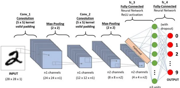
Figure 2.1: Typical architecture of a convolutional neural network and its different layers

CNN architectures consist of many stacked layers (Figure 2.11) where each layer learns diff

er-ent features from the input images. Initial layers usually learn basic features like edges, and the

final layers learn features with higher complexity that uniquely describe the input data.

Con-ventional neural networks consist of an input layer, hidden layers, and an output layer. Each

layer has a specific objective and performs a particular operation, the layers commonly used

are described below.

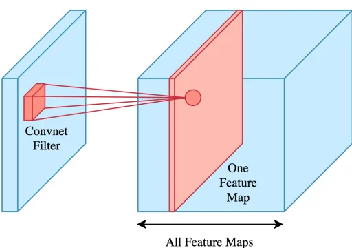
Convolutional layer

The convolutional layer is the principal component of a CNN. It transforms the input data by

applying convolution operations between its associated kernel (also called filter) and a local

region of the input. The objective of this layer is to construct high-level features of the input

image, that later are used to identify patterns such as shapes and can be used in classification

1_{from https://towardsdatascience.com/}

6 Chapter2. Background

or object detection tasks (Figure 2.22).

Figure 2.2: A convolutional layer showing the convolutional operation between its associated filter and the input data

Pooling layer

The pooling layer has the function of reducing the size of the feature maps to reduce the number

of parameters in the final model and control overfitting during the training process. Pooling

layers are commonly placed after the convolutional layer with a down-sampling factor of 2

(Figure 2.33_).

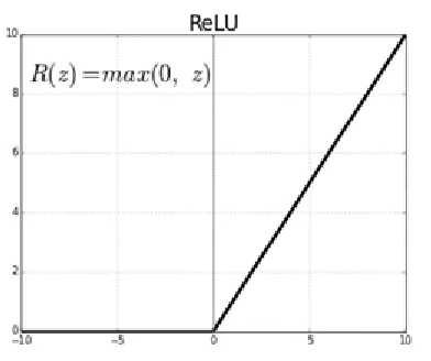
ReLU layer

The ReLU (rectified linear unit) layer applies a non-linear thresholding function to each

ele-ment of a feature map, where the negative values are set to zero, and the positive values have

no variation (Figure 2.44).

2_{from https://towardsdatascience.com/}

applied-deep-learning-part-4-convolutional-neural-networks-584bc134c1e2

3_{from http://cs231n.github.io/convolutional-networks/}

2.1. Convolutional neural networks 7

Figure 2.3: A pooling layer applying a max operation to reduce the size of a feature map

Figure 2.4: ReLU layer and its associated thresholding function applied to the input data

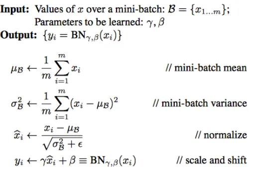
Batch normalization layer

Batch normalization is a technique proposed by Ioffe et al. [12]. This technique addresses

the problem of internal covariate shift by normalizing layer inputs. As is stated in the original

paper, batch normalization permits the use of higher learning rates and also works as a

regu-larizer, reducing the need for Dropout layers [31] that are typically used to reduce overfitting.

8 Chapter2. Background

Figure 2.5: Batch normalization algorithm applied to an inputx.

L2 regularization

Regularization is a technique to control overfitting by adding a penalty term to the loss function.

L2 regularization is the most used form of regularization. It adds the square magnitude of all

parameters as a penalty to the loss function: λP

jw2j. Whereλis the penalty term also known

as regularization parameter or weight decay that determines the amount of penalty added to the

weights of the model.

Softmax classifier

Softmax classifier is a popular multi-class classifier. It uses as activation function the softmax

function, described in the following equation:

fj(z)=

ezj P

kezk

(2.1)

2.2. CNNarchitectures 9

the sum of all its elements is equal to one. The output of the softmax function also represents

the normalized probability that the input feature vectorzbelongs to a particular class j. Figure 2.65) shows an illustration of the softmax classifier.

Figure 2.6: Softmax classifier. For an inputzwith arbitrary scores for each class j, the output is a vector with values between 0 and 1 for each class j.

2.2

CNN architectures

With the increase of computational power and the availability of large datasets, CNNs have

become popular for perform tasks such as image classification. The first successful application

of CNNs is LeNet [14] in 1998 and was used to recognize handwritten and machine-printed

characters. The most popular CNNs architectures that have been used for image classification

in the ImageNet Large Scale Visual Recognition Challenge (ILSVRC) are:

AlexNet

Developed by Alex Krizhevsky, Ilya Sutskever, and Geoff Hinton, AlexNet [13] achieved a

top 5 error rate of 16% on the ILSVRC challenge in 2012. Since its publication, AlexNet has

become a staple in computer vision literature inspiring other successful architectures.

10 Chapter2. Background

GoogLeNet

Developed by work from Szegedy et al. GoogLeNet [35] won the ILSVRC challenge in 2014

with a top 5 error rate of 6.67%, its main contribution is the inception module that uses small

convolution filters allowing the reduction of the number of parameters in the final model.

VGGNet

VGGNet [29] won the second place in the ILSVRC challenge in 2014, because of its

simplic-ity. It is widely used as a feature extractor for other applications such as object detection. With

approximately 140 M of parameters, it requires significant memory and computational power.

ResNet

With a top error rate of 3.57%, ResNet [8] developed by Kaiming He et al. won the ILSVRC

challenge in 2015. It first introduced the concept of “skip connections” that help to reduce the

vanishing gradient problem during the training process.

MobileNet

MobileNet [10] is designed to address computer power limitations in embedded vision

appli-cations. To reduce the number of parameters and the model size, MobileNet uses a depthwise

separable convolution. It achieves similar accuracy values as VGG-16 and GoogleNet with

2.3. ObjectDetection 11

2.3

Object Detection

Object detection is one of the main research areas in computer vision. Its main objective is

to find objects in an image (object localization) and determine the class of the object (object

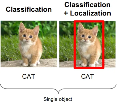
classification) among a predefined set of categories [40] (Figure 2.76).

Figure 2.7: Difference between image classification (left) and object detection (right).

Traditional object detection algorithms follow a typical pipeline that consists of:

Region selection:To find objects in an image, traditional methods scan the entire image

apply-ing slidapply-ing windows of different sizes and scales and generating smaller image crops that later

are analyzed individually to determine if there is an object inside the sliding window. Due to

the significant number of analyzed candidates, this process is computationally expensive [40].

Feature extraction:To analyze each candidate generated during the sliding windows process,

we need visual features that give us meaningful information about the image. Popular visual

features include SIFT (scale-invariant feature transform) features [20] that have the property

of being invariant to image scale and rotation, HOG (histograms of oriented gradients) features

[5] used in human detection and Haar-like features [17] used in face recognition. However,

12 Chapter2. Background

most of the feature descriptors are designed to detect a specific type of objects, and their

per-formance could be affected by illumination conditions.

Classification: Once we have the feature descriptor vector of each sliding window, the next

step is to classify the image crops in a target object class and background. The most common

algorithm used is SVM (support vector machines) [3].

Non-maxima suppression (NMS): Due to the sliding window process many candidates are

generated and to filter the most significant results, non-maxima suppression is performed. Only

the results with the highest scores are selected as the result of the object detector.

Object detectors based on CNNs have become popular due to the success of the application

of CNN architectures (for example VGGNet [29], ResNet [8]) as feature extractors. Object

detectors based in these CNN architectures have achieved state of the art performances in terms

of accuracy and good enough detection speed to be deployed in mobile devices [11]. CNN

networks have the ability to learn more sophisticated features due to their deep architectures,

finding more complex patterns in images. Features learned by CNNs are more robust than

the features manually designed, which makes CNN architectures more suitable for a variety of

applications since we can train the same model with different datasets. [40].

Generic object detectors based on CNNs have the objective of classifying the objects in an

image and show the position of the objects drawing a rectangular bounding box around them.

Generic CNN based object detection methods can be classified into two groups: two-stage

detectors and one-stage detectors.

Two-stage detectors

Two-stage detector frameworks consist of a two-step process. First, the algorithm focuses in to

generate a region of interest or proposals and then classify each region of interest into

prede-fined object classes(Figure 2.8). Successful algorithms in this category are Region-based fully

2.3. ObjectDetection 13

(R-CNN) [27]. In Faster R-CNN a base network (VGGNet for example) is used as a feature

extractor, and features from an intermediate feature map are selected to generate proposals

(300 in the original paper [27]). In the next stage, these feature proposals combined with the

output of the base network are used to predict object classes and bounding box coordinates.

R-FCN [4] follows a similar process compared with Faster R-CNN, but the regions of interest

are generated from the output of the base network instead of an intermediate feature map. This

change reduces the computational power needed, increasing the speed of detection, training

and achieving similar accuracy compared with Faster R-CNN.

Figure 2.8: High-level diagram for two-stage detectors, showing the region proposal phase and the classification phase (image from [11]).

One-stage detectors

One-stage detectors directly predict the object class and location as a regression problem in a

single pass through a convolutional neural network (Figure 2.9). The main objective of

one-stage detectors is to improve the detection speed, however, their accuracy is lower compared

with two-stage detectors.

The most popular algorithms in this category are You only look once (YOLO) [26] and Single

shot multibox detector (SSD) [19]. YOLO divides the input image in an SxS grid, for each

14 Chapter2. Background

and the number of bounding boxes B are hyperparameters of the algorithm. SSD uses default

anchor boxes with different aspect ratios and scales to make predictions in six feature maps,

with the objective of predict objects with different scales and shapes. The network generates

as output, scores for the presence of objects, and bounding box coordinates.

Figure 2.9: High-level diagram for one-stage detectors, showing the one-step process that com-bines classification and bounding box prediction (image from [11]).

2.4

State-of-the-art in Tra

ffi

c Sign Detection

Traditional traffic signs detection algorithms are based on image processing techniques, where

the feature extraction is performed manually. These methods consider the main characteristics

of traffic signs such as specific color and shape. Color based techniques use the color of the

traffic signs as the main feature to identify their location on the image [33]. Supreethet al. [32] use color segmentation to detect red color traffic signs, the images are transformed to grayscale

from RGB color space. Next, the algorithm selects region candidates in the image applying

shape and size constraints, crops and saves the selected regions, and passed them through a

neural network for classification.

Although color segmentation using the RGB space takes less computational power and time,

it is difficult to apply in real time environments because it requires stable illumination

condi-tions. In order to have algorithms less sensitive to illumination changes, Nguwiet al.[22] use the Hue-Saturation-Intensity (HSI) color space to locate road signs and neural networks for

gener-2.4. State-of-the-art inTrafficSignDetection 15

ate candidate regions. HOG features are used as feature descriptors, and an SVM classifier is

used to identify the traffic sign category.

Shape-based segmentation is as an alternative for color-based segmentation. It relies on the

assumption that traffic signs come in a regular shape (rectangle, triangle, circle, octagon).

Nguyen et al. [23] use Hough transform to detect general shapes (circles, rectangles, etc.) and is complemented with edge detection to detect speed limit and warning signs. Yang et al. [37] use a color probability model to generate areas of interest, alongside with Histogram of Oriented Gradient (HOG) features as a feature descriptor, and a CNN performs the

classifi-cation. Zabihi [38] presents a method for detection and recognition of traffic signs inside the

attentional visual field of drivers, HOG features with SVM are used for detection and SIFT

features with color information for recognition.

With the improvement of computational power and the availability of suitable datasets, deep

learning methods have become popular in computer vision tasks. As was mentioned in the

previous section, the main categories for generic object detectors based on CNNs are two-stage

detectors and one-stage detectors. Many traffic sign detectors based on CNNs use variants of

the generic object detectors. Zhang et al. [39] use a modified version of YOLOv2 [24] to detect traffic signs. The authors changed the filters sizes, and the number of layers to find

the best balance between speed and accuracy. M¨uller et al.[21] present another interesting application of one stage detectors (SSD), it uses a deeper feature extractor and modified default

bounding boxes to increase accuracy for traffic lights detection. Zhu et al. [41] designed a CNN architecture considering that traditional object detectors are trained to detect objects

that occupy a significant portion of an image, in contrast, traffic signs usually occupy a small

16 Chapter2. Background

2.5

Evaluation metrics

Intersection over union

Bounding Boxes are evaluated using the intersection over union (IoU) metric also known as the

Jaccard index, which is a ratio between the intersection and the union of the area of predicted

boxes (Apred) and the area of the ground truth boxes (Agt). IoU is the metric used in the matching

strategy to determine if a default bounding box corresponds to the ground truth box or the

background.

IoU = Apred∩Agt Apred∪Agt

Mean average precision (mAP)

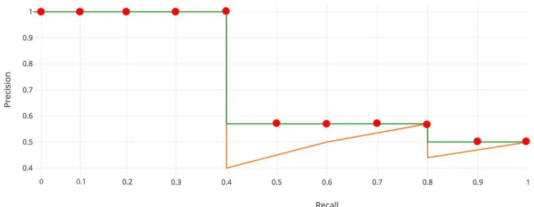
The primary metric of evaluation for object detectors is the mean average precision (mAP). For

the interpolated mAP (Salton and McGill 198) used in the VOC2007 challenge the area under

the precision-recall curve is interpolated at a set of eleven equally spaced recall levels [0, 0.1, .

. . , 1]:

mAP= 1 11

X

r∈{0,0.1,...,1}

pinter p(r)

2.5. Evaluation metrics 17

pinter p(r)= max

˜

r:˜r>r p(˜r)

Where p(˜r) represents the measured precision at a recall value ˜r. As is stated by Everingham et al. [6], interpolating the area under the precision-recall curve reduces the impact of the ”wiggles” in the curve caused by small variations in the ranking of examples. (Figure 2.107_).

Figure 2.10: Interpolated precision-recall curve (green line with red dots) used for the calcula-tion of mean average precision

For the Pascal VOC (Visual object classes) dataset, the metric is calculated for an IoU threshold

of 0.5, for the COCO (Common objects in context) dataset the mAP is calculated as an average

of ten different IoU thresholds from 0.5 to 0.95 in steps of 0.05. Taking an average of ten IoU

thresholds, this method rewards models that have better localization precision.

Chapter 3

Tra

ffi

c signs detector

In this chapter, the methodology used to build the traffic signs detector is presented. The final

experiment results are compared against the generic object detector SSD [19]. SSD architecture

is used as a baseline to deploy the model presented in this thesis.

3.1

SSD architecture review

SSD is designed to make predictions on images in one single pass, the output is expressed in

terms of a set of default bounding boxes and a value of confidence of the presence of the target

object class for each default bounding box. The algorithm makes predictions in six different

scale feature maps in an attempt to identify objects of different sizes and shapes. The main

characteristics of the SSD algorithm are:

Multi-scale feature maps for detection

SSD algorithm adds extra convolutional feature layers at the end of the base network, these

layers decrease in size progressively to make predictions on six different layers (with sizes of

38x38, 19x19, 10x10, 5x5, 3x3, 1x1 using VGG16 [29] as the base network). The algorithm

3.1. SSDarchitecture review 19

Figure 3.1: Comparison between SSD [19] and YOLO [26] network architectures. SSD adds feature layers to the end of a base network and, uses six feature maps to make predictions. YOLO uses one feature map to make predictions.

makes four predictions for the first, fifth and sixth layers and six predictions for the remaining

three layers. YOLO in the other hand makes predictions in one feature scale [26], Figure 3.1

shows the difference between these two architectures.

Default bounding boxes and aspect ratios

SSD [19] associate each cell in the feature maps used for prediction with a set of default

bounding boxes. The algorithm predicts the offsets relative to the default box in the cell and a

confidence score that expresses the presence of a target object class inside the default box. For

kgiven locations in a feature map, the algorithm computescclass scores by applying (c+4)k filters for each feature map cell. For an m× n feature map, the output will have a size of (c+4)kmn. SSD algorithm applies default bounding boxes to all the six feature layers used for prediction. These default bounding boxes have different scales and aspect ratios in order to

efficiently predict objects of different sizes and shapes. Figure 3.2 shows an illustration of how

20 Chapter3. Traffic signs detector

Figure 3.2: Default bounding boxes and aspect ratios in SSD. During training, the algorithm needs the input image and ground truth bounding boxes (a). Anchor boxes of different aspect ratios are defined at each location in feature maps with different scales ( for example 8 x 8 (b) and 4 x 4 (c)) (image from [19]).

Matching strategy

During the training process, the ground truth box needs to be matched with a default bounding

box to train the algorithm accordingly. The ground truth is matched with the default

bound-ing box with the best jaccard index (also known as intersection over union). An overlappbound-ing

threshold of 0.5 is used during the training process, the index values below 0.5 are labeled as

background, and the values higher than 0.5 are labeled as a target object. Authors claim that

this gives the network more flexibility, simplifying the learning process [19].

Training Objective

The loss function used for training is a weighted sum of the classification loss (Lcon f) and the

localization loss (Lloc):

L(x,c,l,g)= 1

3.1. SSDarchitecture review 21

WhereNrepresents the number of matched default bounding boxes. The localization loss is the SmoothL1loss [7] between the predicted (l) and ground truth (g) bounding box parameters. The parameters for each default bounding box (d) are its center (cx,cy), width (w) and height (h). All these values are encoded as shown in the following equations:

Lloc(x,l,g)=

N X

i∈Pos m∈{cx,cy,w,h} X

xk_{i j}smoothL1(lim−gˆ m

j) (3.2)

Where:

ˆ gcxj =

(gcx_j −d_icx) dw

i

ˆ

gcy_j = (g

cy

j −d

cy

i )

dh i

ˆ

gw_j =log(g

w j

dw_i ) gˆ

h

j =log(

gh j

d_ih)

The classification or confidence loss is the softmax loss over all the target classes (c) [19].

Lcon f(x,c)= −

N X

i∈Pos

x_{i j}plog(ˆc_ip)− X

i∈Neg

log(ˆc0_i) (3.3)

where ˆc_ip = exp(c

p i)

P

pexp(c p i)

.

Hard negative mining

Because of the matching strategy, a large number of default bounding boxes are labeled as

background, resulting in a high imbalance between the positive classes (target objects) and

negative class (background). In SSD [19], the training samples are filtered by confidence score,

keeping the most significant ones. In the end, the algorithm always tries to keep a ratio of 3:1

22 Chapter3. Traffic signs detector

3.2

Dataset

For this thesis, the dataset used is the CSUST Chinese traffic sign detection benchmark (CCTSDB)1

[39]. The dataset consists of 10000 images and three categories (or classes): mandatory traffic

signs, prohibitory traffic signs, and warning traffic signs. Each image has an annotation file

that contains the coordinates of the ground truth bounding box and the class ID of the target

object. One or more traffic signs can be included in a sample image. For evaluation purposes,

the dataset was split into 80% for the training set and 20% for the test set.

Figure 3.3: Sample images from the dataset.

3.3

Methodology

Base network selection

With the objective to reduce the computational complexity, training, and detection time, the

selection of the base network is a primary task while building an object detector.

3.3. Methodology 23

art convolutional neural networks [29] [8] [34] have deeper architectures with the objective of

reaching high accuracy values. However, these accuracy improvements come with a decrease

in detection speed, which makes deeper networks challenging to apply in real-world scenarios

where the computational cost is a crucial factor.

MobileNet [10] presents a successful design that efficiently balances network size and speed.

According to the authors, MobileNet achieves an accuracy of 70.6% on the ImageNet

clas-sification dataset. In comparison, VGG-16 [29] achieves 71.6% on the same dataset, but,

MobileNet is 30 times smaller than VGG-16 in terms of the number of parameters. The main

component that makes MobileNet a light architecture is the depthwise separable convolution,

which divides the traditional convolutional layer into two parts: depth-wise convolution and

point-wise convolution. The first part, the depthwise convolution, applies a single filter to each

input channel. The second part, pointwise convolution, applies a 1x1 convolution to combine

the outputs of the depthwise convolution in one result [10] [28]. In comparison, a typical

convolution layer, filters and combines the inputs into a set of outputs in one step (Figure 3.4).

Figure 3.4: Standard convolutional layer (left) versus Depthwise Separable convolution layer (right)(image from [10]).

Figure 3.5 shows the mobilenet architecture, which consists of a traditional convolutional layer

followed by 13 depthwise separable convolutional blocks. Each one of these blocks contains

a batch normalization layer to reduce the internal covariate shift and the risk of overfitting

during training. The last layers that are used for classification tasks are an average pool layer,

24 Chapter3. Traffic signs detector

a feature extractor for object detection, the last three layers previously mentioned (responsible

for classification) were removed, following a similar process used in the SSD paper [19].

Figure 3.5: Mobilenet architecture for classification tasks. It consists on a traditional convo-lutional layer followed by 13 depthwise separable convoconvo-lutional blocks. The last layers are an average pool layer, followed by a fully connected layer and finally, a softmax layer (image from [10]).

Feature maps selection for prediction

As mentioned in section 3.1, SSD algorithm uses six feature maps with different scales to make

predictions. The objective is to tackle a central dilemma of object detectors based on CNNs,

the balance between classification and localization. In CNNs, the last layers have more

se-mantic information, which is useful for classification. However, size reduction of feature maps

3.3. Methodology 25

of small objects. This trade-offbetween localization and classification is the main reason why

SSD algorithm uses feature maps of different sizes. The features maps with higher sizes are

responsible for small object detection. However, features in shallow layers do not have enough

semantic information, which makes the classification part more difficult, resulting in a poor

representation when it comes to small object detection. To avoid this drawback, Liet al.[16] and Cao et al. [2] propose feature fusion modules to form a feature map with more context information to improve small object detection while following the same feature pyramid

struc-ture of SSD. Leeet al.[15], propose residual blocks and deconvolution layers to enrich feature maps of shallow layers with context information from the last layers.

Following these ideas, feature maps of different sizes are combined for the final predictions.

The question now is: which feature layers combine?. For this reason, the feature maps are

plotted for different scales of the SSD algorithm using MobileNet as a base network, showing

only the areas of interest (traffic signs). The idea is to identify which feature map is responsible

for the detection of traffic signs of different sizes.

26 Chapter3. Traffic signs detector

Figure 3.6 shows some results for an input image size of 300x300. As can be seen, the output

of layer of size 75x75 and the layer of size 38x38 can localize the small traffic signs in the

sample images. For the layer of size 19x19, some small traffic signs are missed due to the

typical downsampling process related to CNNs.

As part of the experiments for this thesis, different feature maps are fused and tested to

deter-mine the best combination. One and two feature maps for prediction were tried, measuring the

accuracy and computational cost.

Anchor boxes selection

Anchor boxes are a crucial parameter in one-stage object detectors. The aspect ratio, scale, and

the number of anchor boxes should be carefully selected because they impact the efficiency

and accuracy value of our object detector directly. As mentioned in the previous section, SSD

algorithm utilizes a set of default bounding boxes with different scales and aspect ratios for

each feature map used for detection. For this project, the anchor boxes were selected using the

k-means cluster algorithm with the goal of maximize the value of intersection over union (IoU)

in the predictions. As is stated by Redmonet al.[24], using the Euclidean distance as a metric for the k-means algorithm leads to significant errors as the size of the boxes increases. For this

reason, a distance metric based on IoU is used to determine the clusters [24] [25].

d(box,centroid)= 1−IoU(box,centroid) (3.4)

The number of anchor boxes could be considered as a hyperparameter in the training process.

Selecting a high number of anchor boxes may improve the quality of our predictions in terms

of IoU, but this will also increase the computational cost needed for training and prediction. In

order to select the best number of anchor boxes, the average IoU versus the number of clusters

3.4. Experiments 27

Figure 3.7: Number of anchor boxes vs mean IoU, with six anchor boxes the mean IoU is around 0.75, with ten anchor boxes the mean IoU is around 0.8

As we can see in figure 3.7, the relationship between the number of anchor boxes and mean

IoU is not linear. With six anchor boxes, the mean IoU is around 0.75, and with ten anchor

boxes, we have an IoU around 0.8. To get a mean IoU above 0.85, the number of anchor boxes

needs to be at least 17. For the experiments, six anchor boxes were used in the model with

one feature map for prediction. For the model with two feature maps for prediction, ten anchor

boxes were used, five for each feature map.

3.4

Experiments

For all the experiments a computer with an Intel i7-4829K @ 3.70GHz CPU and a NVIDIA

Tesla K80 GPU was used. The size of the images for all the tests is 300x300. The average

precision (AP) was measured with an intersection over union (IoU) threshold of 0.5. The

com-putational cost was estimated, counting the number of multiplications and additions (MAC)

op-erations [10], which is equivalent to calculate the floating point opop-erations per second (FLOPs)

28 Chapter3. Traffic signs detector

(measured in a GPU) are presented. The predictions per class is a fixed number, and it is

di-rectly proportional to the size of the feature map used for prediction. For a feature map of size

m∗nandkanchor boxes, the number of predictions per class is equal tom∗n∗k.

Data augmentation

Following the training strategies used in SSD [19], we used data augmentation to increase

the number of training samples artificially. The objective is to obtain a better generalization

and robustness in our final model. To each image in the training dataset is applied one of the

following options:

• Use the entire input image.

• Sample a patch with an IoU value of 01, 0.3, 0.5, 0.7, or 0.9 with the target object.

• Randomly crop a patch of size between 0.1-1 of the original image size.

After the sampling step, each patch is re-sized to a fixed size and is flipped horizontally with

a probability of 0.5, in addition to applying some photo-metric distortions such as contrast,

brightness, and color manipulation similar to those described by Howard[9].

Training parameters

The proposed algorithm was implemented using Pytorch 0.4 as framework. The source code is

based on open source repositories (ssd.pytorch2_{and RFBNet}3 _{[30]). The training parameters}

and strategies are similar to the ones used in SSD [19]. Stochastic gradient descent (SGD) was

used as the optimization algorithm with an initial learning rate of 0.001, momentum of 0.9, and

a batch size of 32. With the objective of avoiding overfitting, a learning rate decay policy and

L2 regularization with weight decay (penalty parameter) of 0.0005 were applied.

3.4. Experiments 29

Epochs 250

Batch size 32

Optimizer SGD

Learning rate 0.001

Learning Rate Decay Policy Drop by a factor of 10

at 150 and 200 epochs

Momentum 0.9

Weight Decay 0.0005

Table 3.1: Training parameters used in experiments

Experiment 1

The first round of tests consists of building an object detector with one feature map for

detec-tion. For this purpose, the output of the base network, which has a size of 10x10 (for an image

input of 300x300) is upsampled and concatenated with a feature map of a higher scale. For

this experiment, six anchor boxes are used according to the analysis shown in the methodology

section.

Figure 3.8, shows the network architecture for experiment 1. It consists of three tests. For the

first test, the feature map of size 10x10 is upsampled and concatenated with the feature map of

size 19x19. In the second test, the feature map of size 10x10 is upsampled and concatenated

with the feature map of size 38x38. Finally, in the third test, the feature map of size 10x10 is

upsampled and concatenated with the feature map of size 75x75.

30 Chapter3. Traffic signs detector

Results of experiment 1

The results are presented in table 3.2. The test using the feature map of size 38x38 gives

7.73% higher accuracy and 87.7% more computational cost than the model using the feature

map of size 19x19. The reason could be that the feature layer with a higher size (38x38) has

more fine-grained information necessary to detect small objects than the smaller feature map

(19x19) which is reflected in, the higher accuracy value.

The test using the feature map of size 75x75 has a lower accuracy value compared with the test

using the feature map of size 38x38 (86.13% vs. 86.22%) and is 1.61 ms slower. In this case,

the feature map of size 38x38 gave better accuracy values and is faster. For this reason, test 2

showed the best performance in experiment 1. Comparing test 2 vs. test 3, using a feature map

with a higher size did not increase the accuracy values, it seems that the 75x75 feature map is

too shallow and does not contain enough context information, even when combined with the

upsampled 10x10 feature map.

Layers fused AP, IoU: 0.5 Detection time (ms) # Predictions per class MAC (in millions) Parameters (in millions)

10x10 - 19x19 78.49 7.61 2166 1620 4.87 10x10 - 38x38 86.22 8.04 8664 3040 4.81 10x10 - 75x75 86.13 9.65 33750 8450 4.77

Table 3.2: Results of experiment 1

Experiment 2

The second experiment consists of an object detector with two feature maps for detection.

Figure 3.9 shows the network architecture for experiment 2, which consists of three tests. In

the first test, the feature map of size 10x10 is upsampled and concatenated with the feature

map of size 38x38 for the first feature map for detection. The resulting feature map of size

38x38 is upsampled again and concatenated with the feature map of size 75x75 for the second

3.4. Experiments 31

and concatenated with the feature map of size 19x19 for the first feature map for detection.

The resulting feature map of size 19x19 is upsampled again and concatenated with the feature

map of size 38x38 for the second feature map used for detection. Finally, in the third test, the

feature map of size 10x10 is upsampled and concatenated with the feature map of size 19x19

for the first feature map for detection. The resulting feature map of size 19x19 is upsampled

again and concatenated with the feature map of size 75x75 for the second feature map used for

detection. For this experiment, ten anchor boxes are used, five for each feature map used for

detection.

Figure 3.9: Network architecture for experiment 2

Results of experiment 2

The results of experiment 2 are presented in table 3.3. The second test gives an accuracy value

of 0.25% higher and 66.4% less computational cost than the model used in test 3. Compared

with the first test, the second test gives 2.74% higher accuracy with less than the half

compu-tational cost. Comparing test 2 vs. test 3, test 2 reached better accuracy values and is 2.07 ms

faster than test 3. For this reason, test 2 showed the best performance in experiment 2. Similar

to experiment 1, the feature map of size 75x75 does not add any benefit to the performance of

the model. The lack of context information in the shallow layer of the base network could be

32 Chapter3. Traffic signs detector

Layers fused AP, IoU:

0.5 Detection time (ms) # Predic-tions per class MAC (in millions) Parameters (in millions)

10x10 - 38x38 — 38x38 - 75x75 90.74 14.14 35345 5230 5.29 10x10 - 19x19 — 19x19 - 38x38 93.48 10.08 9025 2200 5.37 10x10 - 19x19 — 19x19 - 75x75 93.23 12.15 29930 3660 5.35

Table 3.3: Results of experiment 2

Experiment 3

For experiment 3, is used the same network architecture as in experiment 2. However, instead

of upsampling and concatenation modules, residual blocks are used. As is stated by Lee et al. [15] and Wang et al.[36], residual feature maps try to maintain low-level information of shallow feature maps while having a high-level abstraction of feature maps of the lasts layers

in the base network. By separating the prediction module from the base network, the gradients

of the prediction module do not flow towards the feature maps of the base network [15].

Fig 3.10-a shows the three-way residual block [15]. It consists of three branches: branch one

reduces the number of channels of the input feature map, branch two increases the

represen-tation power of the shallow feature map through a 3x3 convolution layer, and branch three

makes the upsampling through a deconvolution layer, to propagate context information to a

small feature map [15]. For experiment 3, two tests were made. The first test with the

three-way residual block [15]. The second test with a small change in the method of combining the

branch 3 and branch 1, 2, using concatenation instead of element-wise sum, fig 3.10-b.

Results of experiment 3

The results of experiment 3 are presented in table 3.4. The second test gives an accuracy

value of 0.19% higher, 2.31% more computational cost and is 0.42 ms slower than the model

used in test 1. Both tests in this experiment gave better accuracy values than the best result in

experiment 2. Residual blocks can increase accuracy values, and for this application (detecting

3.4. Experiments 33

(a) Three-way residual block as is presented in [15].

(b) Three-way residual block modified for ex-periment 3

Figure 3.10: Residual blocks used in experiment 3

(better accuracy values with an increase of detection time of less than 0.5 ms).

Test AP, IoU: 0.5 Detection time (ms)

MAC (in millions)

Parameters (in millions)

Test 1 93.56 12.02 3030 7.6 Test 2 93.75 12.44 3100 7.7

Table 3.4: Results of experiment 3

Finally, table 3.5 shows the comparison of the proposed network against the generic object

detector SSD with VGG16 and MobileNet as the base network. The detection speed was

evaluated using a NVIDIA Tesla K80 GPU and an Intel i7-4829K @ 3.70GHz CPU. The

com-putational cost measured in multiplications and additions (MAC) operations is not proportional

to the detection speed. The proposed algorithm has 2.67 times MAC operations than the

SSD-MobileNet algorithm. The SSD-SSD-MobileNet is 1.3 times faster than the proposed algorithm in a

CPU. In an GPU the SSD-MobileNet model is 1.49 times faster than the proposed algorithm.

In terms of accuracy, the proposed algorithm reached a higher value (93.75% vs. 89.35%)

compared with SSD-MobileNet.

Compared with SSD-VGG16, as expected, SSD-VGG16 gives a higher accuracy value because

of the use of a deeper base network. For the same reason, SSD-VGG16 is slower compared

34 Chapter3. Traffic signs detector

Method Avg. Precision, IoU: Detection time MAC Parameters

0.5 0.75 0.5:0.95 GPU

(ms)

CPU (sec)

(in millions)

(in millions)

SSD- VGG16 95.71 86.5 75.12 52.75 1.59 30590 24.01 SSD-MobileNet 89.35 68.82 62.41 8.35 0.337 1160 5.65 Proposed algorithm 93.75 88.79 73.47 12.44 0.438 3100 7.7

Chapter 4

Conclusions and Future work

In this thesis, an adapted version of the single shot multibox detector (SSD) algorithm

mod-ified for traffic sign detection is presented. The base network was changed from VGG-16 to

MobileNet. The reason for this change is to use a lighter network architecture, that efficiently

balances network size and detection speed. A common approach seen in deep learning

lit-erature for increasing the accuracy values in object detection applications is using a deeper

and more sophisticated base network. However, deeper architectures require high

computa-tional power, and in some cases, the detection time is too high that makes them not suitable for

real-time applications. The proposed algorithm has a comparable accuracy value (93.75% vs.

95.71%) compared with the Single shot multibox detector (SSD) algorithm (with VGG-16 as

base network), which means that a light size CNN architecture like MobileNet can be used as

a base network to build reliable object detectors when the computational cost is a limitation.

The number of feature maps used for prediction was reduced, from six in the original SSD

algorithm to two. This change was driven by the fact that traffic signs come in regular shapes

(circle, triangle, and rectangle), and in defined colors. Therefore, they could be detected with

simpler convolutional neural networks (CNN) architectures. In experiment 1 and experiment

2 feature fusion map that combines context information from deeper CNN layers with the

information in shallow layers was used. This is more useful for localization purposes. Different

36 Chapter4. Conclusions andFuture work

feature maps were combined to find the combination that provides the best accuracy value.

During these experiments, feature maps visualization has proven to be a useful tool that helps

to identify the best feature map candidates to combine and also have a better understanding of

how the convolutional layers work. An interesting result during the evaluation process showed

that using feature maps of shallow layers (like the feature map of 75x75), will not necessarily

give the best accuracy values. This result shows that although shallow layers provide useful

information to detect small objects. They do not have enough context information that makes

the classification task more difficult.

Results of experiment 3 showed that residual blocks are a good technique to increase context

information in shallow layers in a CNN. Compared with the results of experiment 2, experiment

3 reached higher accuracy values. However, residual blocks also increase the size, complexity

of the network and, detection time. All of these factors need to be taken into account, especially

if the objective is to use the object detector in real-time applications where the detection time is

crucial. The process followed in this thesis can be used to design object detectors for specific

applications, for example, street light detection, waste bin detection for automatic waste

col-lection systems, applications where the target objects have a regular form and a limited range

of colors.

For future work, the goal is to use LIDAR (Light Detection and Ranging) data as part of a

more robust object detector. Test more low computational cost oriented CNN architectures like

MobileNet-V2 [28] and PeleeNet [36] as base network, following the same design process used

in this thesis. Testing different loss functions, especially the localization loss function is also

planned. In SSD algorithm, Smooth L1 is used as a loss function. This loss function tries to

minimize the distance between the ground truth and the predicted bounding box. However, the

similarity between the ground truth and the prediction is measured through intersection over

union (IoU), a loss function based in IoU could increase the quality of the predicted bounding

boxes and the accuracy values because during the training process the algorithm will optimize

Bibliography

[1] N. Ben Romdhane, H. Mliki, and M. Hammami. An improved traffic signs recognition

and tracking method for driver assistance system. In2016 IEEE/ACIS 15th International Conference on Computer and Information Science (ICIS), pages 1–6, June 2016.

[2] Guimei Cao, Xuemei Xie, Wenzhe Yang, Quan Liao, Guangming Shi, and Jinjian Wu.

Feature-fused ssd: fast detection for small objects. InNinth International Conference on Graphic and Image Processing (ICGIP 2017), volume 10615, page 106151E. Interna-tional Society for Optics and Photonics, 2018.

[3] Corinna Cortes and Vladimir Vapnik. Support-vector networks. Mach. Learn., 20(3):273–297, September 1995.

[4] Jifeng Dai, Yi Li, Kaiming He, and Jian Sun. R-FCN: object detection via region-based

fully convolutional networks. CoRR, abs/1605.06409, 2016.

[5] N. Dalal and B. Triggs. Histograms of oriented gradients for human detection. In

2005 IEEE Computer Society Conference on Computer Vision and Pattern Recognition (CVPR’05), volume 1, pages 886–893 vol. 1, June 2005.

[6] M. Everingham, L. Van Gool, C. K. I. Williams, J. Winn, and A. Zisserman. The pascal

vi-sual object classes (voc) challenge.International Journal of Computer Vision, 88(2):303– 338, June 2010.

[7] Ross B. Girshick. Fast R-CNN. CoRR, abs/1504.08083, 2015.

38 BIBLIOGRAPHY

[8] Kaiming He, Xiangyu Zhang, Shaoqing Ren, and Jian Sun. Deep residual learning for

image recognition. CoRR, abs/1512.03385, 2015.

[9] Andrew Howard. Some improvements on deep convolutional neural network based image

classification. arXiv preprint arXiv:1312.5402, 2013.

[10] Andrew G. Howard, Menglong Zhu, Bo Chen, Dmitry Kalenichenko, Weijun Wang,

To-bias Weyand, Marco Andreetto, and Hartwig Adam. Mobilenets: Efficient convolutional

neural networks for mobile vision applications. CoRR, abs/1704.04861, 2017.

[11] J. Huang, V. Rathod, C. Sun, M. Zhu, A. Korattikara, A. Fathi, I. Fischer, Z. Wojna,

Y. Song, S. Guadarrama, and K. Murphy. Speed/accuracy trade-offs for modern

con-volutional object detectors. In2017 IEEE Conference on Computer Vision and Pattern Recognition (CVPR), pages 3296–3297, July 2017.

[12] Sergey Ioffe and Christian Szegedy. Batch normalization: Accelerating deep network

training by reducing internal covariate shift. CoRR, abs/1502.03167, 2015.

[13] Alex Krizhevsky, Ilya Sutskever, and Geoffrey E. Hinton. Imagenet classification with

deep convolutional neural networks. Advances in neural information processing systems, page 1097–1105, 2012.

[14] Y. Lecun, L. Bottou, Y. Bengio, and P. Haffner. Gradient-based learning applied to

docu-ment recognition. Proceedings of the IEEE, 86(11):2278–2324, Nov 1998.

[15] Kyoungmin Lee, Jaeseok Choi, Jisoo Jeong, and Nojun Kwak. Residual features and

unified prediction network for single stage detection. CoRR, abs/1707.05031, 2017.

[16] Zuoxin Li and Fuqiang Zhou. Fssd: Feature fusion single shot multibox detector. CoRR, abs/1712.00960, 2017.

[17] R. Lienhart and J. Maydt. An extended set of haar-like features for rapid object detection.

BIBLIOGRAPHY 39

[18] Tsung-Yi Lin, Piotr Doll´ar, Ross B. Girshick, Kaiming He, Bharath Hariharan,

and Serge J. Belongie. Feature pyramid networks for object detection. CoRR, abs/1612.03144, 2016.

[19] Wei Liu, Dragomir Anguelov, Dumitru Erhan, Christian Szegedy, Scott Reed,

Cheng-Yang Fu, and Alexander C. Berg. SSD: Single shot multibox detector. ECCV, 2016.

[20] David G. Lowe. Distinctive image features from scale-invariant keypoints. International Journal of Computer Vision, 60:91–110, 2004.

[21] Julian M¨uller and Klaus Dietmayer. Detecting traffic lights by single shot detection.

CoRR, abs/1805.02523, 2018.

[22] Y. . Nguwi and A. Z. Kouzani. Automatic road sign recognition using neural networks.

InThe 2006 IEEE International Joint Conference on Neural Network Proceedings, pages 3955–3962, July 2006.

[23] B. T. Nguyen, S. J. Ryong, and K. J. Kyu. Fast traffic sign detection under challenging

conditions. In2014 International Conference on Audio, Language and Image Processing, pages 749–752, July 2014.

[24] Joseph Redmon and Ali Farhadi. Yolo9000: Better, faster, stronger. arXiv preprint arXiv:1612.08242, 2016.

[25] Joseph Redmon and Ali Farhadi. Yolov3: An incremental improvement. arXiv, 2018.

[26] Santosh Redmon, Joseph and Divvala, Ross Girshick, and Ali Farhadi. You only look

once: Unified, real-time object detection. arXiv preprint arXiv:1506.02640, 2015.

[27] Shaoqing Ren, Kaiming He, Ross B. Girshick, and Jian Sun. Faster R-CNN: towards

real-time object detection with region proposal networks. CoRR, abs/1506.01497, 2015.

[28] Mark Sandler, Andrew G. Howard, Menglong Zhu, Andrey Zhmoginov, and Liang-Chieh

Chen. Inverted residuals and linear bottlenecks: Mobile networks for classification,

40 BIBLIOGRAPHY

[29] K. Simonyan and A. Zisserman. Very deep convolutional networks for large-scale image

recognition. CoRR, abs/1409.1556, 2014.

[30] Di Huang Songtao Liu and Yunhong Wang. Receptive field block net for accurate and

fast object detection. arxiv preprint arXiv:1711.07767, 2017.

[31] Nitish Srivastava, Geoffrey Hinton, Alex Krizhevsky, Ilya Sutskever, and Ruslan

Salakhutdinov. Dropout: A simple way to prevent neural networks from overfitting. J. Mach. Learn. Res., 15(1):1929–1958, January 2014.

[32] Supreeth H.S.G and C. M. Patil. An approach towards efficient detection and recognition

of traffic signs in videos using neural networks. In 2016 International Conference on Wireless Communications, Signal Processing and Networking (WiSPNET), pages 456– 459, March 2016.

[33] M. Swathi and K. V. Suresh. Automatic traffic sign detection and recognition: A review.

In2017 International Conference on Algorithms, Methodology, Models and Applications in Emerging Technologies (ICAMMAET), pages 1–6, Feb 2017.

[34] Christian Szegedy, Sergey Ioffe, and Vincent Vanhoucke. Inception-v4, inception-resnet

and the impact of residual connections on learning. CoRR, abs/1602.07261, 2016.

[35] Christian Szegedy, Wei Liu, Yangqing Jia, Pierre Sermanet, Scott Reed, Dragomir

Anguelov, Dumitru Erhan, Vincent Vanhoucke, and Andrew Rabinovich. Going deeper

with convolutions. InComputer Vision and Pattern Recognition (CVPR), 2015.

[36] Robert J Wang, Xiang Li, Shuang Ao, and Charles X Ling. Pelee: A real-time object

detection system on mobile devices. arXiv preprint arXiv:1804.06882, 2018.

[37] Y. Yang, H. Luo, H. Xu, and F. Wu. Towards real-time traffic sign detection and

classifi-cation. IEEE Transactions on Intelligent Transportation Systems, 17(7):2022–2031, July 2016.

[38] Seyedjamal Zabihi. Detection and recognition of traffic signs inside the attentional visual

BIBLIOGRAPHY 41

[39] Jianming Zhang, Manting Huang, Xiaokang Jin, and Xudong Li. A real-time chinese

traffic sign detection algorithm based on modified yolov2. Algorithms, 10:127, 11 2017.

[40] Zhong-Qiu Zhao, Peng Zheng, Shou-tao Xu, and Xindong Wu. Object detection with

deep learning: A review. CoRR, abs/1807.05511, 2018.

[41] Zhe Zhu, Dun Liang, Songhai Zhang, Xiaolei Huang, Baoli Li, and Shimin Hu. Traffi

Appendix A

Detection examples SSD

+

MobileNet vs.

Proposed Algorithm

(a) SSD+Mobilenet (b) Proposed algorithm

43

(a) SSD+Mobilenet (b) Proposed algorithm

44 ChapterA. Detection examplesSSD+MobileNet vs. ProposedAlgorithm

(a) SSD+Mobilenet (b) Proposed algorithm

Curriculum Vitae

Name: Jose Luis Masache Narvaez

Post-Secondary Escuela Superior Polit´ecnica del Litoral

Education and Guayaquil, Ecuador

Degrees: 2004 - 2009 B.Eng. Electronics and Telecommunications Engineering

University of Western Ontario London, ON

2017 - present, Master of Engineering Science

Related Work Teaching Assistant

Experience: The University of Western Ontario 2019