Formally Assessing Cryptographic Entropy

(1)

Formally Assessing Cryptographic Entropy

Daniel R. L. Brown

∗

January 2, 2013

Abstract

Cryptography relies on the secrecy of keys. Measures of information, and thus secrecy, are called entropy. Previous work does not formally assess the cryptographically appropriate entropy of secret keys.

This report defines several new forms of entropy appropriate for cryptographic situations. This report defines statistical inference methods appropriate for assessing cryptographic entropy.

1 Introduction

Cryptography’s aim is to enable correspondents to communicate securely in the presence of an adversary. The correspondents generally need an advantage over the adversary to secure communication. This advantage almost always includes one or more keys known to at least one of the correspondents but unknown to the adversary. These keys are called secret (or private) keys. Most cryptographic protocols rely on such secret keys because if the adversary knew the secret key(s), then the adversary would know as much as the correspondents and could undermine the security of the protocol.

Secrecy of the keys corresponds to the lack of information that the adversary knows about the keys. Information is measured in entropy. So, the keys must have some amount of secret entropy. In general, the type of entropy appropriate for cryptography is min-entropy, which measures the difficulty of guessing the information (see§3.1.1, [X9.82], or [Lub96]).1 In certain situations, other types of entropy are appropriate for cryptography, such as working entropy (see§3.1.5) and contingent entropy (see§3.2.2).

The entropy needed for secret keys is obtained from a source. Sources that have been used or proposed for obtaining cryptographic entropy include a ring oscillator, a noisy diode, mouse movements, variances in disk read times, or even system process resource usages. Generally, one or more samples are obtained from one or more sources. In many cryptographic systems, these samples are accumulated, using a deterministic process, into something called an entropy pool. An entropy pool may be a concatenation of all the values accumulated, but generally, due to memory restrictions, some compression process is applied. The compression process may be as simple as a group addition, or may involve a cryptographic hash function, or may involve randomness extraction. At some point, a value called a seed is extracted from this pool in order to generate a secret key. Key generation often involves a pseudorandom number generator, which takes as input the seed. All the processing from the source samples to the secret key is deterministic and cannot be deemed to add any entropy, because the deterministic algorithms in a cryptographic system cannot be kept sufficiently secret and because it can be difficult to assess the entropy of an algorithm.

This report formalizes the situation in which the probability distribution of the source is not known exactly. Indeed, it is often unrealistic to assume an exact probability distribution for a given a source. Instead, it is assumed that the source adheres to a probability model, which means that its probability distribution belongs to some known set of probability distributions. By enlarging the assumed set of possible distributions, the assumptions about the source may become more realistic. Given a probability model, statistical inference is applied to assess the cryptographic entropy provided by the source. In particular, samples from the source are observed, and then inferences about the unknown probability distribution can be made. Statistical inference generally infers a subset of the probability distributions within the probability model that best fit the observed sample. The entropy depends on the probability distribution, so inferences made about the probability distribution can be used to make inferences about the entropy. In general, inferences take the form of sets, so for cryptographic applications, prudence dictates to infer the least value of entropy among the inferred set of entropies.

1.1 Further Motivation

This section gives further motivation of how entropy is used and generated in cryptography.

1.1.1 Roles of Entropy in Cryptography

This subsection gives some examples of the role that entropy assessment might play in typical cryptographic appli-cations.

1.1.1.1 Seeding Pseudorandom Number Generators A cryptographic system should typically use a well-seeded and well-designed deterministic pseudorandom number generator to generate random numbers, especially keys. The initial seed provides the cryptographic entropy to the numbers generated.

A well-designed pseudorandom number generator should ensure that the numbers generated

1_{Shannon entropy, another type of entropy often used in communication theory, measures the compressibility of information, which is}

(6)

Formally Assessing Cryptographic Entropy 1.1 Further Motivation

• appear as indistinguishable from uniform as needed,

• cannot feasibly be used to recover the internal state of the pseudorandom number generator,

• cannot feasibly be used, together with internal state of the pseudorandom number generator, to determine past internal states. This is calledbacktracking resistance [NIST 800-90].

These are among the goals of the pseudorandom number generators defined in [NIST 800-90], which, in one case, seem to be met under certain assumptions [BG07].

Remark 1.1.Backtracking resistance can also be necessary for the forward secrecy of key agreement schemes.

Remark 1.2.Unclear responsibility for the proper seeding of pseudorandom number generators can result in major problems. Suppose a manufacturer of cryptographic software implements a pseudorandom number generator but does not provide a source of entropy. If the manufacturer sets the seed to a default value, and if the user of the software mistakenly generates “random” values using this default seed, unwittingly believing that the random number generator includes a source of entropy, then the outputs of the pseudorandom number generator should be considered to have zero entropy.

If a formal assessment of entropy had been done in this example, then this severe failure would have been prevented.

Initial seeding is often done in a fairly ideal setting such as at a manufacturing site. This should enable very thorough entropy assessment.

1.1.1.2 Runtime Refreshment of Pseudorandom Number Generators If the internal state of a deter-ministic pseudorandom number generator is somehow revealed to an adversary, then all its future outputs can be determined by the adversary, unless the pseudorandom number generator is refreshed with new entropy.

The property obtained by frequent refreshing is called prediction resistance in [NIST 800-90] (wherein refreshing is called reseeding). Barak and Halevi [BH05] call this property forward security.

The entropy needed for forward security generally must be obtained during operation in the field. In many cases, entropy in the field should be regarded as scarce. For this reason, entropy assessment is appropriate.

Entropy assessment on the sources that will be used in the field can be done both ahead of time before deployment, and also done during operation in the field.

Remark 1.3.It has been pointed out in [JJSH98,BH05], that runtime entropy assessment can risk leaking information to the adversary. As far as possible, such leakage should be incorporated into the entropy assessment, by considering contingent entropy. See§6.1.12for a simplified example.

1.1.1.3 Prospective and Retrospective Assessment A sample from a source can be used to infer something about its distribution. In some cases, the sample is just discarded, and the inference about the source is used to assess its future ability to generate entropy. This approach is prospective assessment. Prospective assessment is most easily handled when the probability model is such that future samples from the source will be independent and identically distributed.

In other cases, the sample is also used for some cryptographic application, such as forming some of the input used to derive a secret key. Reasons for using the observed sample, rather than discarding it, include that entropy is believed to be so scarce that is not affordable to discard it, and that the probability model does not assume independence of future sample values. In this case, the assessment isretrospective.

Remark 1.4.Retrospective assessment can leak information to an adversary, so contingent entropy must be assessed in this case, as noted in Remark1.3.

In complex systems, entropy assessment may be a mixture of both prospective and retrospective assessment.

(7)

For example, in many forms of public-key cryptography, a public key determines uniquely its corresponding private key. As another example, consider a typical stream cipher, which generates a one-time pad from a fixed length key. (An example of a stream cipher is the Advanced Encryption Standard used in counter mode, abbreviated as AES-CTR). Suppose that the one-time pad is used to encrypt a message, part of which is known to the adversary and part of which is unknown. If the adversary knows enough of the message (sufficiently more than the fixed-length key), then, given unlimited computation, the adversary could determine the key and then decipher the whole message (by employing the stream cipher and key in the same way as do the intended correspondents).

By contrast, some cryptographic protocols offer information-theoretic security. Shannon’s one-time pad is the most famous example. These protocols attempt to resist an adversary with unlimited computational power. To achieve this, they often require a very large cryptographic key, which in many cases needs to be nearly uniform. This requirement often makes these protocols impractical.

Keys whose continued security rely on computational assumptions generally have the property ofconfirmability. An adversary who has the candidate key can confirm the key’s correctness by observing the actual use of key. This means that what one considers as the entropy of key must account for an adversary who will exhaustively search for keys. The notion of working entropy from§3.1.5can account for this.

1.1.1.5 Full and Partial Entropy Keys Some types of computational-security keys, such as public keys, permit purely computational attacks which are strictly faster than exhaustive search of all possible values of the keys.

For example, discrete logarithm keys, such as those used in Diffie-Hellman key agreement or ElGamal signatures, may be positive integers less than some prime q. Algorithms, such as Pollard’s rho algorithm, can compute the private key in about√qsteps. Schnorr [Sch01] gives strong evidence that, if the private key is chosen from a random set of size√q (which allows for exhaustive search of √q steps), no significant improvement of generic algorithms, such as Pollard rho, can be any faster than about√q steps. In other words, discrete logarithm private keys seem only to require about half as much entropy as the bit length.

For other types of computational-security keys, such as symmetric encryption keys, the best known computational attacks have cost similar to exhaustive search. For example, consider the block cipher defined in the Advanced Encryption Standard with a key size of 128 bits, abbreviated as AES-128. The best known attacks on AES-128 exhaustively search each possible key, requiring, on average, one half of 2128 _{evaluations of AES. Accordingly,}

AES-128 is generally claimed to provide AES-128 bits of security. But providing AES-128 bits of security seems to require that the key be (almost) uniform, meaning that it has (almost) 128 bits of entropy. Claims of 128-bit security for a 128-bit-key block cipher have created an enormous incentive to generate the key as close to uniform as possible. Creating a nearly uniform distribution by transforming the samples of a highly non-uniform distribution may be rather difficult or costly, because the techniques to produce near uniformity often require some pre-existing source of uniformity, and also because these techniques tend to discard much of the entropy from the non-uniform source.

As an alternative, suppose that AES-128 was used with keys having only 100 bits of entropy. In this case, at most 100 bits of security would be provided. Some chance exists that such keys could be weak. But this would seem unlikely if the keys were selected pseudorandomly, such as by the output of a hash. If 100 bits of security provides adequate protection, then the burden of producing a uniform key is lifted, and one can concentrate on providing adequate entropy.

Although the alternative approach above does not offer the same claim of 128-bit security as does the conventional approach, if the entropy is assessed more accurately in the alternative approach, then the alternative may offer more security than a conventional approach. If a conventional approach aims for uniformity at the cost of underestimating entropy, then it would provide less than the claimed 128 bits of security.

Even in the case of block cipher, entropy is more important than uniformity.

1.1.1.6 Third Party Evaluation When a first party supplies a cryptographic product to a second party, the second party values a third party evaluation, such as [FIPS 140-1], of the cryptographic product. Third party evaluations of entropy have some difficulties:

(8)

third party direct access to the entropy source, without compromising the overall security of the cryptographic product.

• The first party has an incentive to supply the output of a deterministic pseudorandom number generator as the claimed source. To a third-party evaluator, the effect of this would be that the source appears to adhere to a uniform distribution.

1.1.1.7 Organization-Level and User-Level Entropy An organization may wish to provide its members with secret keys for encryption purposes, but to retain a backup copy of the secret keys. In this case, the organization might use a deterministic pseudorandom number generator to generate all member secret keys. The organization may need to be quite sure about the security of the secret keys, so would likely invest considerable resources into using sufficient entropy for the seed.

Some cryptographic applications, such as personal privacy and non-repudiation, require that a user’s secret key be truly secret to the user. In this case, some entropy for the user’s secret key must be generated on the user’s local system.

1.1.1.8 Passwords User-remembered passwords are values that a user must recall and enter into a device, usually to authenticate access to certain privileged information. Such passwords are typically too short to contain enough entropy to be used as a cryptographic secret key in the sense of being able to render exhaustive search infeasible. This shortness is partially based on the belief that users will not remember high-entropy passwords.

Because of low password entropy, any data value which would allow off-line confirmation of password guesses, such as the hash of a password or a simple challenge-response transcript, should be kept private. If these values were public, an off-line exhaustive search could be mounted. Password-authenticated key agreement schemes, such as SPEKE, are designed to avoid such off-line attacks. (The restriction on the exposing of user-remembered passwords to off-line guessing attacks applies to both user-selected and system-generated passwords.)

Despite such usage restrictions, passwords still need some entropy in order to avoid on-line guessing attacks, where an attacker can confirm password guesses on-line. To thwart on-line password attacks, usually a limit on the number of failed password attempts is enforced.

Formally, the notion of working entropy, see §3.1.5, can be used to reconcile the differing levels of entropy between passwords and cryptographic secret keys in a more complex system. Working entropy is defined in terms of a parameter called workload quantifying the number of guesses at the secret that adversary can confirm. If off-line confirmation of passwords is stopped, then the effect is that an adversary trying to guess the password is restricted to a low workload. Other cryptographic secrets, such as public keys, usually are such that the adversary’s workload is only limited by the amount of computation that the adversary can perform.

So, in a complex system, the working entropy of all the secrets can be targeted above some minimum level, say 30 bits, which represents a probability of 2−30 _{of the adversary compromising the system. Some cryptographic}

secrets, including most conventional cryptographic keys, are exposed to off-line attacks so should may have their working entropy assessed at high workload, say of 98 bits. (Uniform 128-bit keys have 30 bits of working entropy at a workload of 98 bits.) Other cryptographic secrets, such as passwords, may be protected in such a way to limit the adversary’s workload, for example to 3 bits (for example by limiting a maximum number of failed password attempts to 7). In this case, passwords may undergo entropy assessment, and perhaps some stringent restrictions, assuming some probability model for passwords, such that a working entropy of 30 bits can be obtained (at a 3 bit workload).

1.1.2 Entropy Source Examples

This report concerns the assessment of cryptographic entropy sources. For the sake of concreteness, some examples of entropy sources, upon which the techniques of this report could be applied, are briefly discussed.

(9)

processor time each has used, contains some entropy. For example, some processes may need to write to a hard disk, and disk seek times are known to vary depending on where data is located on the hard disk and upon other factors.

An advantage of such entropy sources is the lack of special hardware or user action.

1.1.2.2 Environmental Conditions Some systems have inputs which could be used as an entropy source. For example, a microphone can monitor the sound in the local environment.

An advantage of such an entropy source is the lack of special hardware or user action. A possible disadvantage is any adversary close enough may also have partial access to, or control over, the entropy source.

1.1.2.3 User Inputs A user often supplies inputs to system, such as mouse movements or keyboard strokes. These inputs may be used as an entropy source. The inputs used for entropy may be gathered incidentally through normal use, or through a formal procedure where the user is requested to enter inputs with the instruction to produce something random.

In addition to treating user inputs as an entropy source, a system often relies directly on a user to provide a secret value, in form of a user-selected password, as in§1.1.1.8.

Passwords still require entropy, so entropy assessment of user-selected passwords is still warranted.

System-generated passwords generally apply a deterministic function to the output of the random number gener-ator. The deterministic function transforms the random value to a more user-friendly format, such as alphanumeric. The result is still a password which needs some entropy, but in this case, the source of entropy could be some other entropy source instead of user input. The entropy still needs assessment.

1.1.2.4 Coin Flipping Perhaps the archetypal entropy source is the coin flip. A coin is thrown by a person into the air, with some rotation about an axis passing nearly through a diameter of the coin. The coin is either allowed to land on some surface or to be caught in the hand. The result is either heads or tails, determined by which side is facing up.

Coin flips are often modeled such that each result is independent of all previous results. Furthermore, for a typical coin, it is often modeled that heads and tails are equally likely. A sequence of coin flips can be converted to a bit string by converting each result of head to a 1 and each tail to 0. In this simple model, the resulting bit string is uniformly distributed among all bit strings of the given length.

More skeptical models may be formulated. Firstly, it may be noted that a dishonest coin flipper could potentially cheat in certain ways. For example, the cheater may not rotate the coin on the correct axis, but rather an axis at 45◦to the plane of the coin, which may cause the coin to appear to rotate, but always maintain one side closest to a particular direction in space. For another example, a skilled cheater may be able to toss the coin with a given speed and rotation (of proper type) such that either the coin can be caught with an intended side up, or perhaps land on a surface with higher probability of landing on an intended side.

If one considers that cheating is possible, then one should also consider the possibility that an honest coin flipper may inadvertently introduce bias into the coin flips. Indeed, in a cryptographic application relying only on coin flips for entropy, a user may need to flip a coin at least 128 times. As the user becomes tired of repeated flips, the user may start to become repetitive and perhaps suffer from such bias.

To account for this, one could formulate a more pessimistic probability model for the coin flipping, and then do some statistical analysis comparing the pessimistic model with the actual sample of coin flips.

1.1.2.5 Dice Dice, usually as cubes with numbers marked on the faces, have long been used in games of chance. Provided that adequate procedures are used in the rolling, the number that ends up at the top of the die, when its motion has ceased, is believed to at least be independent of previous events.

On the one hand, the roll of a die, once it is released, seems governed mainly by the deterministic laws of mechanics; and so it may seem that all the randomness is supplied by the hand that rolled the die. On the other hand, it seems apparent that the rollers of dice cannot control the results of the die rolls;2 _{and so, it would seem}

that the rolling process itself contributes to randomness.

2_{For example, otherwise, many games of chance would be adversely affected. That such games of chance still seem to work suggests}

(10)

The following explanation may account for this discrepancy. Each collision of the die with the ground causes it to bounce. Because the die is tumbling as it bounces, some of the rotational energy of the die may be converted into translational energy of the die, or vice versa. This conversion depends very much on the orientation of the die as it impacts the surface upon which it rolls. With each bounce, the resulting translational energy affects the amount of time before the next bounce. The amount of time between bounces affects the amount of rotation of the die, and therefore its orientation. This may mean that a small difference in orientation at one bounce results in a large difference in orientation at the next bounce. It may be that a butterfly effect applies. Each bounce may magnify the effect of orientation and rotation, so that the outcome of the die roll, as determined by the final orientation of the die, depends on the extremely fine details in the initial orientation and motion of the die. Such processes are known as chaotic processes. Although technically deterministic, chaotic physical processes are hard to predict, partly because it is too difficult to obtain the necessary precision on the initial conditions to determine the final condition. Rolling dice may be a practical way to seed a random number generator that will be used to generate organizational level secret keys. Rolling dice may be fairly impractical for user-level secret keys, and is infeasible for runtime sources of entropy.

1.1.2.6 Ring Oscillator Ring oscillators have been studied as sources of entropy. See, for example, Sunar, Martin and Stinson [SMS07] or Baudet, Lubicz, Micolod, and Tassiaux [BLMT11].

Ring oscillators are essentially odd cycles of delayed not-gates. Whereas even cycles of delayed not gates can be used for memory storage, ring oscillators tend to oscillate between 0 and 1 (low and high voltage) at a rate proportional to the number of gates in the oscillator.

Since the average oscillation rate can be calculated from the number of gates and general environmental factors, such as temperature, it is only the variations in the oscillation that should be regarded as the entropy source.

Ring oscillators are not always available in general purpose computer systems. But they can be included in custom hardware, or even in field programmable gate arrays (FPGA).

Remark 1.5.Neither [SMS07] nor [BLMT11] explicitly use the approach of this report.

1.1.2.7 Radioactive Decay Some smoke detectors use the radioactive element americium which emits alpha particles. The same method could perhaps be used as a cryptographic entropy source, such as for the generation of organization-level secret keys.

1.1.2.8 Hypothetical Muon Meter For the purposes of hypothetical discussion, consider an entropy source in the form a muon3_{meter. The muon meter provides a 32-bit measurement of the speed of each muon passing through}

the device. On average, one muon passes through the detector per minute. Because of the underlying physics of muons, this entropy source may be viewed as providing a very robust entropy source, whose rate of entropy cannot be reduced by an adversary. 4

This hypothetical source illustrates the task of assessing entropy. Consider the following situation. A crypto-graphic module testing lab receives a vendor submission of such a muon-based source. The lab accepts the general theory supplied by the vendor that each muon 32-bit speed measurement is an independent random variable with some stationary probability distribution. The lab spends about one work day to obtain 1024 speed measurements from the submitted muon detector. All speed measurements are distinct except for a single pair with the same speed. This hypothetical example is treated formally in§6.3. For a simplified analysis, consider the following. Artificially assume that the muon speed measurements are uniformly distributed within some fixed, but unknown, subset of all

3_{A muon is an elementary particle in the standard model of physics. Essentially, it is heavier version of an electron. Muons are a}

form of ionizing radiation, so are easily detectable, and were discovered even before the neutron. Muons are deemed difficult to produce artificially, but do occur naturally on Earth, originating from background cosmic rays (high energy protons) colliding with atoms in the atmosphere. They travel near light speed. Because of their speed and mass, they are highly penetrating, and are detectable through hundreds of meters of rock. Muons are fairly frequent at ground level

4_{This entropy source may succumb to an attack if an adversary surrounds it by other muon detectors, in which case it may be able}

(11)

Formally Assessing Cryptographic Entropy 1.2 Previous Work

possible 32-bit speed measurements. Even more simplistically, further assume just three hypotheses:5 _{that this}

subset has size 210_{, 2}30_{or 2}20_{. In the first hypothesis of a 2}10_{-uniform distribution, one would have actually expected}

many more repetitions than just one. In the second hypothesis of a 230_{-uniform distribution, one would not have}

expected repetitions. In the third hypothesis of a 220_{-uniform distribution, one expects about one repetition after 2}10

samples. Therefore, the third hypothesis seems, at least intuitively, to be most consistent with the sample collected.

Remark 1.6.In the formal view of this report, what this simplistic analysis has done is: assume a formal probability model, although an artificial one; gather a sample; use a sample statistic (§5), namely the a number of repeated elements in the sample sequence; make a statistical inference (§4), using maximum likelihood inference as induced by the chosen sample statistic. The resulting inference is that the distribution with 220 _{possible values is the most likely of the three distributions in the model.} In this case, the inference gives a single maximal distribution, so the inferred entropy can be computed directly from this. See §6.3.5.1for a more detailed treatment.

1.1.2.9 Quantum Particle Measurement The theory of quantum mechanics implies that quantum parti-cles, such as photons or electrons, can exist in a superposition of states under which measurement causes a wave function collapse. The theory states that wave function collapse is a fully random process independent of all past events in the universe. Under this theory, an entropy source derived from such wave function collapse would be totally unpredictable no matter what expense the adversary took to predict the source, a property highly useful for cryptography.6

Jenneweinet al.[JAW+₀₀_{] devised such a device using an attenuated light source, a beam splitter and two single} photon detectors.

1.2 Previous Work

Past publications do not seem to assess cryptographic entropy with adequate formal justification. This subsection gives a brief survey of the most relevant past results.

1.2.1 Hypothesis Testing

Much past work on the assessment of randomness in cryptography, such as [FIPS 140-1] and [Mau90], has taken the form of hypothesis testing. Hypothesis testing fails to assess cryptographic entropy in several respects:

1. Zero-entropy values can be contrived that pass given hypothesis tests, such as taking the output of secure stream cipher or pseudorandom number generator (say one defined in [NIST 800-90]). If contrived zero-entropy values can pass hypothesis tests, then it is possible that zero-entropy, or insufficient-entropy, values can accidentally be generated that pass tests.

2. The outcome of a hypothesis test is binary: it is either a pass or afail, not a quantity of formally assessed entropy.

3. In the formal framework of this report, conventional hypothesis testing of cryptographic random number gener-ators usually consists of using statistical inference in the uniform probability model of§2.3.1. The assumption of the uniform model is problematic because of the following.

(a) It is generally a too strong and unrealistic assumption, which does not attempt to model any realistic deviations from uniformity.

(b) It is subject to the tying effect Remark5.7 which requires the use of sample statistics to overcome tie-breaking effects. Poorly-chosen sample statistics rely on poorly-formulated assumptions about potential divergences from a uniform distribution.

5_{Each of the three hypotheses is an instance of the subuniform probability model discussed in}_§2.3.1_{, but taking all three together can}

be considered as a restriction of the independent probability model in§2.3.2.

(12)

Formally Assessing Cryptographic Entropy 1.2 Previous Work

(c) It is a singular model (§2.3.1), admitting only one probability distribution, so that inferring the distribu-tion, and hence the entropy, is trivial. Once the uniform assumption has been made, all that can really be done is to assess the plausibility of the assumed entropy.

Some developers of “true” random number generators have relied on hypothesis testing in the following way. They build an entropy source with some tunable parameter. For certain values of the tunable parameter, the source may fail the hypothesis tests. For other values of the tunable parameter, the source may pass the hypothesis. The developers tune the parameters such that the entropy source has desirable properties (perhaps efficiency) and such that it passes the hypothesis tests. The entropy of such an entropy source has not been formally assessed.

Although hypothesis testing in cryptography has mainly been applied to the uniform model, it can be applied to any model, and as such can serve purposes other than entropy assessment. Hypothesis testing is further discussed in an appendix to this report§C.

1.2.2 Randomness Extraction

Other past works in cryptography, such as [JJSH98], have studied how to extract almost uniformly random bit strings from random but biased bit strings. This process is calledrandomness extraction(though uniformity extraction would have been a more appropriate term).

Randomness extraction does not solve the problem of assessing entropy. In fact, randomness extraction can only sensibly be applied after entropy assessment, since randomness extraction takes as input values with a sufficient amount of entropy.

In the general framework of this report, the entropy obtained after randomness extraction is defined as applied entropy §3.2.1. In systems that apply randomness extraction in an effort to obtain uniformity, entropy can still be assessed even under assumed probability models that are insufficient for the randomness extraction to produce uniformity.

1.2.3 Entropy Assessment

The following previous works comment on entropy assessment.

1.2.3.1 ANSI X9.82-2 The ANSI accredited standards committee X9’s working group F1 recognized the need for entropy assessment. Working group F1 began draft American National Standard (ANS) X9.82-2 [X9.82] that covers entropy sources. The author was a member of the working group F1 during this time, although not an editor of ANSI X9.82-2. The content of [X9.82] varied considerably as it was edited and as the working group discussed it. No versions of ANS X9.82-2 formalized a notion of a probability model which is a feature of this report (§2). Instead drafts of ANS X9.82-2 mention specific probability models. One draft mentions the hidden Markov model (see§2.3.4for a description of this model), but this was later removed. Later drafts restrict the probability model to the independent identically distributed model (see§2.3.2in this report).

Statistical inference is used in various drafts ANSI X9.82-2. For example, maximum likelihood estimates, with a requirement on large sample size, is used. Hypothesis testing is also used, based on somewhat arbitrary sample statistics, to test the hypothesis of the independent (and identically distributed) probability model.

The ANS X9.82-2 targets not only developers of entropy sources but also third party assessors, such as crypto-graphic module testing laboratories, who have generally reported results as pass or fail.

1.2.3.2 Barak and Halevi Barak and Halevi [BH05] state:

... entropy estimation in general is an inherently impossible task.

The context in which they claim impossibility of entropy estimation may not be the same as the context in which [X9.82] and this report attempt to assess entropy. Nonetheless, the strength of their statement seems to contradict at least the beliefs of the X9F1 working group.

(13)

Formally Assessing Cryptographic Entropy 1.3 Overview of this Report

very low static estimate for the entropy (e.g. such as 1/2 entropy bit per sample [bit]),

which seems inconsistent with their previous statement about the inherent impossibility.

1.3 Overview of this Report

1.3.1 Contributions

The main contributions of this report are:

• formalization of probability models for application to cryptography,

• several new forms of entropy appropriate for cryptography,

• statistical inference methods appropriate for assessing cryptography entropy in a general setting, and

• an entropy assessment paradigm making clear the assumptions upon which the assessment depends.

1.3.2 Organization

The subsequent sections cover the following topics:

• Section 2gives formal definitions and examples of probability models.

• Section 3gives formal definitions of cryptographic entropy.

• Section 4gives formal definitions and examples of general statistical inference.

• Section 5gives formal definitions and examples of sample statistics and the resulting induced inference.

• Section 6provides some examples of assessing entropy.

• Appendix Adiscusses various results from optimization theory which may be applicable to inference methods.

• Appendix Bdiscusses briefly some approaches to formulating a suitable probability model.

• Appendix Cdiscusses the special case of hypothesis testing.

• Appendix Ddiscusses the case where the adversary can influence the probability distribution.

• Appendix Ediscusses estimation theory, a method to assess any given inference method.

(14)

Formally Assessing Cryptographic Entropy

2 Probability Models

Shannon founded information theory, including cryptography, on probabilities. Per Shannon’s theory, in this report, the adversary’s lack of information is described in terms of probabilities. This report further tackles the dilemma that the cryptographer does not necessarily know these probabilities. So, the cryptographer makes formal assumptions about the probabilities, in the form of aprobability model, which is defined in this section.

Once the probability model is assumed and a sample from the source is observed, statistical inference, see§4, can be used to assess of cryptographic entropy, see§3, provided by the source.

Many different probability models can be formulated under the notion of this report. Statistical inference depends on choice of probability model. Because the formal entropy assessment in this report is stated with respect to a probability model, the formal assessment of entropy includes the full description of the probability model. Re-iterating, an assessment of entropy is not formal unless it specifies a formal probability model.

A formal entropy assessment is only as appropriate as the probability model is appropriate for the given entropy source.

Remark 2.1.In this report, probabilities are used to measure an adversary’s pre-existing lack of knowledge about a value which the adversary wishes to guess. An adversary may acquire extra knowledge about a specific value, which leads to the modifications of the entropy defined in§3.2, such as contingent entropy from§3.2.2 which accounts for an adversary having extra information about the outcome of a probabilistic event. Conversely, the cryptographer may have more knowledge than the adversary regarding a specific source sample, in which case eventuated entropy from§3.3.2can be used to account for an adversary having less information about the probabilistic event than the cryptographer has.

2.1 Formal Definition of Probability Models

A probability space Π and asample space X are sets. In cryptographic contexts,X is usually finite but Π is often uncountably infinite. The sample spaceX will be assumed to be finite, unless otherwise noted. An elementp∈Π is called aprobability distribution, or just adistribution, for short. An element ofx∈Xis called asample. Aprobability function for Π andX is a function

P : Π×X →[0,1] : (p, x)7→Pp(x), (2.1)

where [0,1] is the interval of real numbers between 0 and 1 inclusive; and the functionP is such that for allp∈Π, the following summation equation holds:

X

x∈X

Pp(x) = 1. (2.2)

Aprobability model is a triple (Π, X, P), where Π is a probability space,X is a sample space, andP is a probability function.

Remark 2.2.For given p∈Π, writePp for the function such thatPp:X →[0,1] :x7→Pp(x). When clear from context, the

functionPpmay also be called a probability function.

Remark 2.3.For the task of assessing entropy, probability theory notions of an event and a random variable do not play a significant role, for the following reasons.

• Aneventcorresponds to a subset ofX, and a probability distribution defines the probability of an event. IfXis discrete, andE⊆X, then the probability of the event, under distributionp, isP_x∈EPp(x), using this report’s formalism for a

probability model. Because only discrete sample spaces are relevant to cryptography, the notion of an event is derivable from the formal definition of a probability model, and is thus redundant.

Usually entropy depends on the probability of a single sample, not the probability of an event. The notion of an event is incorporated into the definitions of certain kinds of entropy, such as eventuated entropy from§3.3.2, but the formal definition of probability can be stated without reference to the notion of an event.

• A random variable is a variable taking values in the sample space X, with probabilities given by a given probability distribution p. If X is discrete, then notions such as the expected value of random variables can be expressed as

P

x∈XPp(x)xusing this report’s formalism of a probability model. Because only discrete sample spaces are relevant to

(15)

Formally Assessing Cryptographic Entropy 2.1 Formal Definition of Probability Models

Usually entropy depends on the probability of a single sample, not on the expected value of a random variable. Indeed, generally the values of samples have no bearing on the entropy.

A possible role for the notion of random variables is in non-categorical probability models, see§2.5.3, where the sample values have structure that is useful in making statistical inference by way of sample statistics§5.

Remark 2.4.In cryptography, the notationP(x) is often used for the probability of an eventX occurring. In the notation of this report, a subscriptphas been added to reflect the fact that the probability distributionpis an unknown variable.

Remark 2.5.In cryptography, the adversary is also modeled. Three relations between the adversary and the distribution to be inferred are:

1. The adversary does not know the distributionp. 2. The adversary knows distributionp.

3. The adversary chooses the distributionp∈Π.

The three levels grant the adversaries successively more power.

Remark 2.6.This report mainly focuses on the second level adversarial model, where the adversary knows p, because this model is the most important and realistic.

Remark 2.7.The first level adversary, which is more optimistic for the cryptographer than the second level, can be treated formally as an instance of the second level if the adversary’s lack of knowledge about the distributions in the first level can be formulated in terms of probability. This would result in a new model at the second level, in which the distributions formally model the distributions of the first level, combined with a distribution on the distributions. See Remark2.61 for an example.

Remark 2.8.In contrast to the adversary, the cryptographer does not knowp, but instead tries to inferp. So, the adversary actually has more power than the cryptographer. This may be realistic if the adversary has more access to the entropy source and can spend more effort on better statistical inference.

Remark 2.9.Over and above knowing the distributionp, an adversary may also be able to learn some information about a samplexdrawn from the distribution fromp. This can be accounted by using contingent entropy§3.2.2.

Remark 2.10.The third level adversary from Remark2.5is discussed briefly in§D. In this case, the probability model is not controlled by the adversary, only the probability distribution. However, in the formalism of choosing a probability model, the model should be chosen to encompass all the possible distributions which the adversary may be able to invoke. The formalism need not give the adversary influence overx, which the adversary can already influence by influencingp.

Remark 2.11.Cryptography deals with finite or discrete sample spaces X. Nevertheless, sometimes it is useful to consider continuous sample spacesX, such as a precursor model which gets subjected to a discretizing transformation. Working in the continuous model may actually simplify statistical inference, because the discretizing transformation may be discontinuous and non-smooth, making it awkward to optimize (optimization arises in the statistical inference process).

Remark 2.12.WhenX is a continuous space, equipped with a measureµ, then (2.2) is replaced by

Z

X

Ppdµ= 1, (2.3)

and furthermore, the range of the probability function is extended as follows:

P: Π×X →[0,∞] : (p, x)7→Pp(x), (2.4)

so nowPp(x) can exceed one. In this case, the functionPp:X→[0,∞] :x7→Pp(x) is called aprobability density function.

Remark2.13.In greater generality,Xneed not have a pre-existing measure. Instead, letM(X) be the collection of all measures onX. Then the model is defined by some function

(16)

Formally Assessing Cryptographic Entropy 2.2 Equivalence, Isomorphism and Restriction

with the condition: _Z

X

dµp= 1. (2.6)

In the previous example,µp=Ppµheld. In the case of a finite or countably infinite setX, then the measureµpcan be defined

from the usual probability functionPpvia

µp(Y) =

Z

Y

dµp=

X

y∈Y

Pp(y). (2.7)

2.2 Equivalence, Isomorphism and Restriction

If (Π, X, P) is a probability model then two probability distributionsp, q∈Π areequivalent in the model (Π, X, P) ifPp(x) =Pq(x) for allx∈X, which can be writtenp≡q.

Given two probability models (Π, X, P) and (Θ, Y, Q), the models are isomorphic if there exists functions β : Π → Θ and γ : Θ → Π and a bijective function b : X → Y such that for all (p, x) ∈ Π×X it is true that

Pp(x) = Qβ(p)(b(x)) and for all (q, y) ∈ Π×Y it is true that Qq(y) = Pγ(q)(b−1(y)). If one simply relabels the

elements of probability space and the sample space, one obtains an isomorphic model.

Remark 2.14.Entropy, see§3, of a probability distributionpis invariant under isomorphism. Therefore, strictly speaking, from a cryptographic perspective, it suffices to consider probability models only up to isomorphism. That said, certain probability models may include the possibility of numeric relationship between components ofx, in which case, an arbitrary isomorphism would render this relationship arbitrary, and possibly more difficult to process, and in particular, to make inferences about.

Henceforth, models will be considered only up to isomorphism, unless otherwise noted.

Remark 2.15.If (Π, X, P) is probability model and z ∈X is such thatPp(z) = 0 for all p∈ Π, then z is said to be

non-occurring. Otherwise zwill be said to beoccurring. Modifications of models by addition or removal of non-occurring sample values may be considered weakly isomorphic.

Given two probability models (Π, X, P) and (Θ, Y, Q), the latter is arestriction of the former if Y = X and Θ⊂Π and, for allp∈Θ andx∈Y, it is true thatQp(x) =Pp(x). Conversely, (Π, X, P) is arelaxation of (Θ, Y, Q).

Similarly, (Θ, Y, Q) is more restrictive than (Π, X, P), and (Π, X, P) is less restrictive than (Θ, Y, Q).

If (Π, X, P) is a probability model, and p∈ Π and x, y ∈X and Pp(x) =Pp(y), then xand y are said to be

equiprobable at distributionp.

Remark 2.16.Equiprobable distributions have equal typicality,§4.4.2.

Ifxandy are equiprobable at allp∈Π, thenxandy are said to beequilikely in the model.

Remark 2.17.All non-occurring sample values are equilikely.

Remark 2.18.Likelihood functions are defined in§4.4.1. Equilikely sample valuesxandyhave the same likelihood functions:

Lx=Ly.

2.3 Examples of Models

Statistical inference can be conducted over any probability model. For the sake of concreteness, some example models are given in this section.

2.3.1 Singular, Uniform, and Deterministic

A probability model (Π, X, P) issingular if|Π|= 1, so that probability space contains just a single distribution. A singular model is the most restrictive model possible, with the exception of adegenerate model which has an empty probability space, so|Π|= 0.

An example of a singular probability model is theuniformprobability model wherePp(x) = 1/|X|for allx. More

(17)

Formally Assessing Cryptographic Entropy 2.3 Examples of Models

there is a uniform model onX, which will be written asu(X). Up to isomorphism, the uniform model is determined by the cardinality of X, so this uniform model may be referred to as the |X|-uniform model. For example, the 6-uniform model implies a uniform model with|X|= 6, a model sometimes assumed for a single roll of a cubic die. When clear from context, uniform is applied to distributions, not just models. Specifically, for any probability model (Π, X, P), a distributionp∈Π is the uniform distribution ifPp(x) = 1/|X|for allx∈X. If (Π, X, P) contains

a uniform distribution, then it is a relaxation of the uniform modelu(X).

Remark 2.19.The uniform distributionpis generally the most cryptographically secure probability distribution on the sample space, because it has the maximum possible min-entropy, log₂|X|(see§3.1.1), of all distributions on the spaceX, and because it is usable as one-time pad.

Another important example of a singular probability model is adeterministic model. In this case, Π ={p} and there is somex0∈X, such thatPp(x0) = 1 andPp(x) = 0 ifx6=x0.

As with the term uniform, when clear from context, the term deterministic applies to individual probability distributions, not just models. Specifically, if (Π, X, P) is a model,p∈Π, andPp(X) ={0,1}, thenpis a deterministic

distribution. Ifpis deterministic andPp(x) = 1, then the notationp=px will sometimes be used, i.e.,Ppx(x) = 1

andPpx(y) = 0 fory6=x.

Remark 2.20.A deterministic distribution is the least cryptographically secure distribution, because a deterministic distribu-tion has zero min-entropy, see§3.1.1, which means that an adversary knowing the distribution can guess the sample value.

Remark 2.21.For a given probability model, it is worth being well aware of the set of deterministic distributions that it contains, since when one obtains a sample valuexsuch that the deterministic distribution onxbelongs to the model, inferring that the distribution could be deterministic is very compelling. Samplexand deterministic distributionpx are as perfect a fit

between a sample and distribution as can be. In this case, a prudent inference method infers an entropy of zero.

Remark 2.22. Apseudo-deterministicmodel is a model that contains a deterministic distributionpxfor eachx∈X. Inference

in a pseudo-deterministic model can be problematic, because, given samplex, the distributionpxis the best inference, which

is deterministic and has zero entropy. Any inference method that includes px among the inferred set of distributions to be

made from x, and takes the minimum min-entropy of the inferred distributions as the inferred entropy, gives an inferred min-entropy of zero. So, a prudent inference method infers zero entropy, no matter what sample is observed, if the assumed model is pseudo-deterministic.

Remark 2.23.A fatalisticmodel on a sample spaceX is the most restricted pseudo-deterministic model: Π ={px :x∈X},

withPpx(x) = 1 andPpx(y) = 0 fory6=x. The fatalistic model is also the least restricted model in which all distributions have zero min-entropy.

The fatalistic model is more pessimistic than a deterministic model, or any other of its proper restrictions, because the fatalistic model cannot be rejected by hypothesis testing. For example, if a deterministic model with Π ={px}is wrong, then

it is possible that a sample obtained can bey withy 6=x, in which case the model will be seen to have been wrong. The fatalistic model, even if incorrect, does not admit such rejection.

The fatalistic model is more pessimistic than any of its proper relaxations, even though these models are also pseudo-deterministic, because no inference method, even an overly optimistic, imprudent method, can sensibly infer a positive value for the entropy.

Assuming a fatalistic model is assuming an omniscient adversary, such as fate, without granting the cryptographer any foresight about the source.

Assuming some model that is not fatalistic can be empirically justified if, upon scrutiny by a real adversary, the adversary gains no advantage, unless the adversary conceals this advantage. A formal justification for a non-fatalistic model for an entropy source is successful hypothesis testing of an alternative fatalistic model. A more intuitive justification of a non-fatalistic model for a source would be that the source has uses wider than just for cryptography and that the prediction of the source would confer some advantage that nobody seems able to obtain.

Remark 2.24.Intermediate to uniform and deterministic models are a family of singular probability models calledsubuniform

models. For integersm, N with 16m6N, a (m, N)-subuniform model is such that|X|=N, andPp(x)∈ {0,1/m}for all

x∈X, which implies thatPpis nonzero on a subset of cardinalitym, and that it is constant on this subset. TheN-uniform

(18)

Similarly, subuniform distributions are distributionspin any probability model (Π, X, P) such thatPp(X) ={Pp(x) :x∈

X}={0,1/m}, for some integerm.

Remark 2.25.Singular models, especially the uniform model, have been used in hypothesis testing, as in [FIPS 140-1]. Statistical inference, see§4, is the process of inferring something about pfrom a given value ofx. In a singular model, only one value ofp is possible. The inference to be made in a singular model therefore takes the form of a pass or fail, or perhaps some grading of the fit between an observed samplexand the model’s single distribution.

Singular models are generally inappropriate for assessing cryptographic entropy, because they generally already assume a value of the entropy and because the limited form of the inference (pass or fail).

Remark 2.26.Even if the uniform model is plausible for some source, such as the entropy source devised by Jenneweinet al.

[JAW+₀₀_{], and even if hypothesis testing is one’s only goal (say, for some reason, one is not trying to formally assess entropy),}

then the uniform model is still somewhat unsuitable in a formal sense, as is discussed below.

An unsuitably of the uniform model, in a formal sense, is that the uniform model requires the use of sample statistics, see§5, to overcome the tying effect in uniform distributions, see Remark 5.7. As such, sample statistics, when applied to hypothesis testing, are essentially trying to detect the possibility that the hypothesis is false. In other words, the sample statistic is testing if some other hypothesis is more realistic. But sample statistics do not formally state what the alternative hypothesis is.

This report therefore proposes an alternative approach to modeling and hypothesis testing, which is outlined in§6.5,§B and§C.

2.3.2 Independent (Identically Distributed)

Another probability model is the (m, N)-independent (identically distributed)model:

Π =np= (p0, . . . , pm−1) :pi∈[0,1],

X

pi= 1

o

= [0,1]m1 (2.8)

X ={x= (x0, . . . , xN−1) :xi∈ {0,1, . . . , m−1}}=NNm (2.9)

Pp(x) = N−1

Y

i=0

pxi. (2.10)

In the abbreviated notations given above: [0,1] means the interval of real numbers between 0 and 1, inclusive; Nm

means{0,1, . . . , m−1};Sm_{means the set of}_m_{-tuples with entries in}_S_{; and}_Sm

1 means the subset ofSmsuch that

the sum of the entries in them-tuple is one.

The parametermis called thewidth, and the parameterN is called thelength. A distribution in (m, N) may be referred to as anindependent distribution on the sample spaceNN

m.

In this model, the parts xi ofxare restricted to be individual random variables withidentical and independent

distributions. There is no restriction, however, on the common distribution.

Remark 2.27.The (m, N)-independent model is a relaxation of themN_{-uniform model because taking} _p_{= (1}_{/m, . . . ,}₁_/m₎

causesPp(x) = 1/mN for allx∈X.

Remark 2.28.In reference to this model, the distribution p may sometimes be called a probability vector, and xcalled a sample vector.

Remark 2.29.The (2, N)-independent probability model may be an appropriate way to model a coin tossed N times if the coin’s probabilities of landing heads or tails are independent and stable.

Remark 2.30.The independent model is also a relaxation of the deterministic model in the following sense. Fix some i ∈ {0, . . . , m−1}. If pi = 1, then Pp(x) = 1 if x = (i, i, . . . , i) and otherwise Pp(x) = 0. These are the only deterministic

distributions in the independent model.

Remark 2.31.ForN>2, the independent model is not pseudo-deterministic.

(19)

Remark 2.33.Given the (m, N)-independent model, it is natural to consider the following functionf :X →[0,1]m defined by the relationf(x)i=|{j:xj =i}|/N. This is thefrequency function, and it is easily seen to be the maximum likelihood

inference (§4.3.1 and§4.4.1) ˆp(x) forx.

Also,Pp(x) is a function off(x), so iff(x) =f(y), thenxandyare equilikely. Furthermore,xandyare equilikely only

iff(x) =f(y).

The number of different values thatf takes is`m+N−1

m

´

= (_mm_!(+_N−N−_1)!1)!. Form≫N, this number is approximately mN−1 (N−1)!, so the average size of an equilikely class is about (N−_m1)!. For N ≫m, the number of values thatf takes is approximately

Nm

m!, so the average size of an equilikely class is about

m!mN

Nm .

Remark 2.34.Randomness (uniformity) extraction is a known method in cryptography, an example of which follows. Suppose that (Π, X, P) is an (m, N)-independent model and thatfis the frequency function defined above. Define a functiong:X→Z as follows: g(x) is the index ofx amongst the list of y withf(y) =f(x), with the list being sorted lexicographically. Let

e(x) = (f(x), g(x)), and letY = [0,1]m_×_Z_{. Then}_e_:_X_→_Y _{is an injection. Define a probability model (Π}_{, Y, Q}_{) such that}

Qp(e(x)) =Pp(x) for all x∈ X. The probability model (Π, Y, Q) is partially subuniform in the following sense: for a fixed

f∈[0,1]m_{, the set}_{_Q

p(f, g) :g∈Z}contains zero and has cardinality at most two. As such, what one can do isextract the

valueg(x) fromx, and essentially ensure that it appears to abide by the uniform model, of a size that may be calculated from

xusing multinomial coefficients. During the process, considerable valuable entropy contained in xmay be lost because the functiongis not injective, with the gain in uniformity usually being a theoretical goal. Entropy is often more important than uniformity, and in some systems, entropy is too scarce to sacrifice.

Remark 2.35.Uniformity extraction can be more generally viewed as taking advantage of the presence of equilikely sample values. Given a sample valuex, one may know that, in the assumed probability model, thatxis equilikely with some number of other sample values. It follows that the index ofxamong this set of equilikely values has a uniform distribution.

Remark 2.36.A relaxation (Π′_{, X, P}′_{) of the independent model (Π}_{, X, P}_{) can be formed by taking Π}′ _{= Π}_×_Σ

X where

ΣX is the set of all permutations ofX. Then let P(′p,s)(x) =Pp(s(x)). This relaxation allows an arbitrary structure on the

sample space, where the structure is the division of each sample in X into a sequence of elements. The distributions which are independently and identically distributed with respect to some arbitrary sequential structure assigned to the elements of

X belong to this relaxed model. Let us call this model thestructureless independent model.

This relaxed model has many equivalent distributions. For example, iftis any permutation of the setNmand is adapted

toXby application to each entry, and adapted to Π by re-ordering of the entries, then (p, s)≡(t(p), t◦s). It may be that for almost all of the space Π′_{, the latter equivalences determine the entire equivalence classes, since the function}_P′

(p,s) determines (p, s) up to the transformation bytas described above, but there are exceptions. For example, if pcorresponds the uniform distribution onNm, then (p, s)≡(p, t) for any permutationsandtofX.

This structureless independent model is pseudo-deterministic, so inference of non-zero entropy in this model is infeasible. However, a (common) product (as in§2.4.5) of structureless independent models may not be pseudo-deterministic, allowing distributions with non-zero entropy to be inferred.

2.3.3 Markov

Another probability model commonly considered is the (m, N)Markov model. The sample space isX=NN m, which

is the same as in the (m, N) independent model. The probability space Π has elements that are pairsp= (v, M), consisting ofv:{0,1, . . . , m−1} →[0,1] whose values sum to one, andM :{0,1, . . . , m−1}2_→_[0_,_{1] whose values,}

when summed with any fixed first argument, total to one. More compactly, Π = [0,1]m

1 ×([0,1]m1 )m. The functions v andM can be viewed as a vector and a matrix, respectively. Then

Pp(x0, . . . , xN−1) =v(x0)M(x0, x1)M(x1, x2). . . M(xN−2, xN−1). (2.11)

This allows xi+1 to depend onxi according to the matrix M. As in the independent model, the parameterm will

be called the width and the parameterN will be called the length.

Remark 2.37.The (m−1, N) Markov model is a restriction, up to isomorphism, of the (m, N) Markov model.

(20)

Remark 2.39.WhenN= 2, the Markov model is isomorphic to the unrestricted model, see§2.3.5, on its sample space, which means that all possible distributions, up to equivalence, are allowed.

Remark 2.40.The deterministic distributions in the Markov model’s probability space are those that take constant valuesx

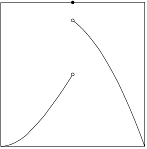
such thatx has the form u(vw)yv ∈ X, where y is a non-negative integer, where ab indicates concatenation of sequences, and where the sequenceuvwhas no repeated elements. Such a sequence may be visualized as aρ, an image familiar to most cryptographers, in which the subsequenceucorresponds to the tail of theρand the subsequencevwcorresponds to the cycle.

Remark 2.41.In the (2,4) Markov model, the distributions (0,1,0,0) and (0,0,1,0) are equilikely. More generally, in the (2, N) Markov model, define a functionf:X→Z3_{, such that}

f(x) = x0,

N−_X1

i=0

xi, N−_X2

i=0

|xi−xi+1|

!

. (2.12)

Iff(x) =f(y), thenxandyare equilikely. A function with the same property for the (m, N) Markov model is given in§5.5.

Remark 2.42.Any source may be viewed as a measurement of a physical process. The elements of a sequence sample in the Markov model may represent individual measurements, such as those taken over time intervals, ideally regular time intervals. In reality, it is generally impossible to measure all the parameters of a physical system that determine its future outcome. For example, the Heisenberg Uncertainty Principle seems to imply this. So the Markov model is not very realistic in that one measurement is not entirely dependent on the previous. Nevertheless, one may hope that, for certain sources, the other true dependencies are effectively predicted by a random variable as provided by the Markov model.

Remark 2.43.The Markov model is not invariant under reversal of the elements in the sample sequence. More formally, the Markov model has no automorphism whose action on the sample consists of reversing the order of the elements in the sequence. More intuitively, the irreversibility of the Markov model can account for cause-and-effect-under-a-rule between consecutive elements of the sequence.

Remark 2.44.Perhaps some type of source is reversible in the sense that the distribution of a source of this type always adheres to some reversible Markov distribution. If the reversibility of that type of source can be firmly established (perhaps by using the inference methods of this report), then a source of that type can modelled by a restriction of the Markov model in which only reversible distributions are included in the probability space. Making such a restriction may perhaps improve the quality of infernce that can be made about the source, and perhaps even raise the inferred entropy.

The fact that many physical laws of motion are invariant under time-reversal may make the reversibility of some sources at least plausible. For example, suppose the sequence elements are obtained from some closed physical process under equal time intervals. If the physical process has no significant external influences, then it may justifiably be deemed as reversible.

Large physical systems are subject the laws of thermodynamics, which include the effect of thermodynamic entropy of a closed system increasing with time. In other words, large closed systems are generally not reversible. At a lower level, the increasing nature of thermodynamic entropy is only a statistical effect, with the underlying physical laws being reversible, but very sensitive and thus chaotic. The chaotic nature means the laws, even if deterministic will result in large changes in the system from minute differences in the initial conditions. The increase in thermodynamic entropy is a statistical effect in the sense that these chaotic effects tend to create a disorganized system, and if even the system is large, its macroscopic parameters will tend to average values of the parameters. For example, organized motion, in the form of kinetic energy will become disorganized motion in the form of thermal energy.

So, the only source that might be well-modelled by a reversible restriction of the Markov model are very small, closed physical systems, whose parameters can be measure without signficance of the influence of the system.

Remark 2.45.For an example of the irreversibility of the Markov model, consider the (2,3) Markov model (Π, X, P) and the distribution p = (v, M) with v = (1,0) and M = (0 1

0 1). This is a deterministic distribution, always taking sample value

x= (0,1,1), sincePp(x) = 1.

For x′ = (1,1,0), the reverse of x, and every distribution p′ = (v′, M′) ∈ Π the probability Pp′(x′) 6 1₄, because

Pp′(x′) =v₁′M₁′_,₁M₁′_,₀ =v₁′M₁′_,₁(1−M₁′_,₁)6(1₄ −(1₂ −M₁′_,₁)2). Therefore, no automorphism of the model can preserve the probablities under the reversal transformation.

Remark 2.46.Certain distributionsp= (v, M) in the (m, N) Markov model (Π, X, P) may be reversible in the sense that there exists areversedistributionp′_{= (}_v′_{, M}′₎_∈_{Π in the model, which is any distribution}_p′_{with the property that}_P