A Modified RANSAC Method for Three-Dimensional Scattering Center Extraction at a Single Elevation

Modified RANSAC Method for Three-Dimensional Scattering

Center Extraction at a Single Elevation

Qinglin Zhai1, Jiemin Hu1, *, Xingwei Yan1, Ronghui Zhan2, Jianping Ou2, and Jun Zhang2

Abstract—In this paper, we focus on the 3D SC model reconstruction from data with wide azimuthal aperture at a single elevation. Since the existing method is difficult to implement for high-frequency signal or large-size target, we propose a modified RANSAC method for the extraction. In our approach, the 3D positions of the SCs are estimated from the 1D SCs via a modified RANSAC method. Then the scattering coefficients are refined via a linear least squares algorithm. The approach is robust with noise because the RANSAC method is able to tolerate a tremendous fraction of outliers. Moreover, it does not suffer from limited accuracy caused by the discretization of the parameter space in [13]. Experiments demonstrate the effectiveness of the proposed approach.

1. INTRODUCTION

In high frequency scattering region, the response of an extended target is well approximated as a sum of responses from a discrete set of points on the target, called scattering centers [1–3]. The scattering

centers can be depicted completely by its positions, scattering coefficients, and types. Therefore,

they provide a concise and physically relevant description of the target radar signature. However,

the scattering centers are sensitive to target pose [4]. In order to solve this problem, the global

scattering center (SC) model is proposed, in which the amplitude attribute of each 3D scattering center is preserved to make the model valid over a large angular extent [5, 6]. The global SC model can be used in numerous radar applications, such as SAR/ISAR imaging simulation [7–9], SAR automatic target recognition [10, 11], etc.

To build the global SC model, different kinds of approaches have been used in previous works. These methods fall into two categories, namely, local 3D based technique [5] and 1D-3D based technique [6]. In the first category, the global SC model is obtained by combining many local 3D SC models at different viewing angles, where each local 3D model requires a large data amount.

In the second approach, the global SC model is obtained by processing the 1D SCs at different viewing angles. Since there are no 2D or 3D imaging steps in model building, the original data amount is not very demanding. In [6], the global SC model is built by repetitiously seeking the highest valued cell in parameter space, which is obtained by applying the Hough transform to the intermediate data called 1D-2D/3D scattering map (OTSM) map. However, the parameter space, constructed via several 3D transformations, needs updating for each SC extraction, which means that the method is terribly time consuming. In [12], we have recently developed a method to extract the global SC model. In this method, the candidate positions are extracted by an accumulator array at the same time, and the parameter-space updating is unnecessary. However, the step of the accumulator array forming is still time consuming.

Received 5 February 2016, Accepted 7 May 2016, Scheduled 2 June 2016

* Corresponding author: Jiemin Hu ([email protected]).

1 _{Electrical Engineering Department, National University of Defense Technology (NUDT), Changsha, China.} 2 _{ATR Laboratory,}

In the previous works, the wide-band measurements in different azimuths and elevations are required. However, in real situations such as the turntable measurement in an anechoic chamber, dense grid and wide coverage in azimuth are easily achieved, whereas the grid in elevation, even if it is sparse, is hard to achieve. In [13], a method is proposed to reconstruct the 3D SCs at a single elevation. The circular aperture is subdivided into a series of overlapped narrow sub-apertures for local 2D SC extraction. The location variation of the scattering centers caused by projection is explored to associate them with a fixed scatterer on the target and to estimate its 3D position. However, the azimuth spacing for local 2D SC extraction must satisfy Nyquist sampling theorem. The relationship between azimuth spacing and signal parameters will be derived in Section 5, which informs that in the applications for Ka or Ku band, or large targets such as warship, the grid is so dense that it is hard to achieve. In order to solve this problem, we try to find a more effective method for 3D SC extraction from the data in a wide azimuthal aperture at a nonzero depression angle.

The 1D-3D based procedures require much less data amount than the local 3D based technique;

therefore, the 1D SCs at different aspects are applied to extract 3D SCs. However, 1D SCs are

estimated from wideband measurements. Some outliers will be produced by the algorithm, especially under low SNR conditions, which is a major obstacle in 3D SC extraction. The RANSAC (Random Sample Consensus) algorithm [14] is a simple, yet powerful, technique commonly applied to the task of estimating the parameters of a model, using data that may be contaminated by outliers. Due to its ability to tolerate a tremendous fraction of outliers, the RANSAC procedure has been widely used in the computer vision community [15, 16]. In this paper, we propose a modified RANSAC method for the 3D SC extraction. The main features of our work are as follows.

1) The 1D SCs extracted at different aspects are viewed as the data that contain outliers, used for 3D SC extraction. Local 2D/3D SC extraction is unnecessary.

2) Due to the capability of the RANSAC algorithm, the proposed method outperforms the existing method under low SNR conditions.

3) Though the 3D SCs are extracted at a specific elevation angle, they are also valid at adjacent elevation angles.

The organization of this paper is as follows. In Section 2, the mathematical formulation of a returned signal at different aspects is described, and the principle of our methodology is introduced. In Section 3, the proposed method to extract the 3D SCs is investigated in detail. In Section 4, the performance of the new method is analyzed. In Section 5, the proposed approach is compared with previous approaches, and some conclusions are drawn in the last section.

2. PROBLEM FORMULATION

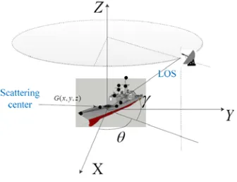
The target coordinate system is depicted in Fig. 1. It is well known that the electromagnetic field scattered from a target can be approximated as a discrete set of SCs on the target, which can be

expressed as [6]

E(f, θ, γ) = K

k=1

ak(θ, γ)

f f0

_αk

exp [−j4πf(x_kcosγcosθ+y_kcosγsinθ+z_ksinγ)/c] (1)

wherecis the speed of light,θthe azimuth angle,f the instantaneous frequency,f0the central frequency

of signal, andγ the elevation angle, anda_k(θ, γ) the scattering coefficient ofkth SC. It should be noted

thata_k(θ, γ) varies with aspect angle (θ, γ), which means that a_k(θ, γ) is a function of the aspect angles

(θ, γ). The type parameterα_k depends on the scatter’s local geometry according to the GTD theory [1].

According to [6], it is very difficult to correctly identify the type parameter unless the signal-to-noise (SNR) is sufficiently high. Furthermore, its effect on the reconstructed scattering data is not notable when the relative bandwidth is not very large [6]. Therefore, it is not considered in this work. In

Equation (1), K is the number of SCs. {x_k, y_k, z_k} denotes the location of kth SC. At an aspect angle

of (θ, γ), the projective 1D location ofkth SC can be calculated as

rk(θ, γ) =xkcosγcosθ+ykcosγsinθ+zksinγ. (2) The parameters of a 3D SC model can be represented as [12]

U={A_k, x_k, y_k, z_k} k= 1, ..., K (3)

whereA_k is aP ×Qcomplex matrix storing the scattering coefficients of the kth SC, i.e., the element

ak,p,qin thepth row andqth column denotes the scattering coefficient at azimuthθ_p and elevationγ_q. P

andQrepresent the numbers of azimuth and elevation grid points. In this paper, the data are collected

at a nonzero depression angle, which means that Q= 1, and elevation γ_q can be simplified asγ.

According to Equations (1) and (2), parameters of thek-th SC in a 1D SC model can be expressed

as {a_k(θ, γ), r_k(θ, γ)} where (θ, γ) denote the aspect of the line of sight (LOS). It is noted that the

parameters in a 1D SC model express the projective information at (θ, γ). For a SC, the parameters in

a 3D SC model are constant; while the parameters in the 1D SC models vary with aspects. In Equation

(2), {a_k(θ, γ), r_k(θ, γ)} can be estimated from the wideband measurements at (θ, γ), and θ and γ are

available beforehand. However, the 1D SC models only depict projective 1D location of the SCs, the

3D positions of the global SCs are not available, i.e., x_k, y_k and z_k are unknowns. In this paper, we try

to use the 1D location of the SCs to generate the 3D positions of the SCs.

If we takex_k, y_k andz_kas model parameters which can be estimated from the sample datar_k(θ, γ),

three samples are enough for model extraction. This can be described as follows:

_r

k(θ1, γ)

rk(θ2, γ)

rk(θ3, γ)

=

_cosγcosθ

1 cosγsinθ1 sinγ

cosγcosθ2 cosγsinθ2 sinγ

cosγcosθ3 cosγsinθ3 sinγ

xk

yk

zk

Hd_k (4)

where r_k(θ1, γ), rk(θ2, γ) and rk(θ3, γ) represent three samples of projective 1D location at different

aspects, respectively. In Equation (4), d_k = [x_k, y_k, z_k]T denotes the 3D location of the kth SC to be

estimated. According to Equation (4), we have

d_k =H−1

_r

k(θ1, γ)

rk(θ2, γ)

rk(θ3, γ)

(5)

Eq. (5) shows that the 3D location of a SC can be calculated via three projective 1D samples of the SC at different aspects.

However, some difficulties arise in practical applications, due to the character of radar signal

processing. For example, r_k(θ, γ) is estimated from wideband measurements. The precisions of the

algorithms may affect the results seriously. Especially under low SNR conditions, some outliers are produced and the performance deteriorates dramatically. Another difficulty is that the correspondence among the SCs at different aspects is difficult to establish. In [6], the regular variation among the SCs is exploited using the OTSM map. However, the OTSM map is obtained by a 3D transformation on all the projective 1D samples at different aspects, which is time consuming.

The aim of our work is to extract U, which contains 3D location and scattering-coefficient matrix

of each SC, i.e., d_k andA_k. Here, we estimate these parameters sequentially: The RANSAC algorithm

is applied in 3D positions extraction, to solve the outlier problem. After that, A_k is estimated by a

3. METHODOLOGY

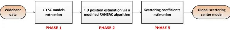
In [13], local 2D SC models are used for 3D SC model extraction. However, the azimuth spacing for local 2D SC extraction must satisfy Nyquist sampling theorem. For the signal in Ka or Ku band, the azimuth spacing is so dense for large targets that it is hard to achieve. In this paper, we use 1D SC models to generate the 3D SC model. The advantage of this method is that the Nyquist sampling theorem is not needed to be satisfied in azimuth spacing. The frame of the extraction methodology is illustrated in Fig. 2. The processing chain is composed of three steps, as shown by the three dashed-line boxes in the figure. In the first phase, the 1D SC models at different aspects, which contain projective 1D location, are extracted from the wideband measurements. In the second phase, the 3D positions of the SCs are estimated from the 1D SC models via a modified RANSAC method. This will be explained in Section 3.2. In the last phase, the wideband measurements are used again to estimate the scattering coefficients of the SCs. The final output is a scattering center model, including not only the 3D position but also the scattering coefficient matrix for each scattering center. Some key steps will be further explained in the following subsections.

Figure 2. Flow chart of the 3D SC model extraction algorithm.

3.1. Estimation of 1D SC Parameter

According to Equations (1) and (2), we have

E(f, θ, γ) = K

k=1

ak(θ, γ) exp [−j4πfrk(θ, γ)/c]. (6)

The objective of this step is to estimate from measurements a set of constant parameters upon which

the received signals depend, i.e., estimating a_k(θ, γ) and r_k(θ, γ) from Equation (6). The principle of

this step is estimating parameters of multiple superimposed exponential signals, which is similar to direction-of-arrival estimation [17, 18], and many super-resolution algorithms are available, such as the structure total least norm (STLN) algorithm [19], the matrix pencil (MP) method [20], the multiple signal classification (MUSIC) algorithm [18], estimation of signal parameters via rotational invariance techniques (ESPRIT) [17], and compressed sensing (CS) based algorithm [21]. Generally, most of them have good performances. Therefore, this paper focuses on extracting the 3D SC model from 1D SC models. It should be noted that, though only the data of HH polarization is used in this paper, and the data of other polarization can be jointly utilized to estimate the 1D SC Parameter [22], with the purpose of suppressing the negative effect from noise.

3.2. 3D Position Estimation via a Modified RANSAC Algorithm

The second step of this methodology is the estimation of 3D position using 1D SCs generated from the first step. Although a lot of previous publications have focused on the first step, we believe that the second step is very crucial for accuracy and robustness of 3D SC extraction. Some false SCs will always exist in the results of the first step. These will act as outliers and hinder accurate estimation of 3D positions if they are estimated by Equation (4). We need robust estimation to overcome the effects of outliers and achieve correct 3D positions.

are estimated from this subset. The model is then evaluated on the entire data set and its support (the number of data points consistent with the model) is determined. This hypothesize-and-verify loop is repeated until the probability of finding a model with better support than the current best model falls below a predefined threshold. However, this approach is limited by the assumption that a single model accounts for all of the data inliers.

In this application of 3D position estimation, each SC can be viewed as an instance of a model, which means that the data contain multiple instances of the same structure. On this occasion, the inliers of one structure behave as pseudo-outliers to the other structures, thus the robust estimator must tolerate both gross outliers and pseudo-outliers, which complicate the problem. Herein, we describe a novel scheme based on RANSAC algorithms to deal simultaneously with multiple models.

As mentioned above, 1D SC parameters include θ, γ, r_k(θ, γ) and a_k(θ, γ). The former three

parameters are used in this estimation. First of all, we put the 1D SCs together as the set of all data,

which can be denoted as D ={x1 x2 . . . xi . . . xI}, where I is the total number of the 1D SCs

(or called points in RANSAC algorithms). In order to obtain a more concise result the ith 1D SC is

represented as x_i= [r_i θ_i γ_i]T where r_i,θ_i and γ_i denote the corresponding 1D location, azimuth and

elevation, respectively. According to Equation (3), there areK models the dataD.

The modified RANSAC scheme is described by the following steps.

Step B-1: Construct a 4×J matrix and set all the elements to zero. This matrix is used for the

multiple model storage: Each column stores major parameters of a model, i.e., 3D position and the

number of inliers. Herein, J denotes the number of models to be stored, which should be larger than

K. The updating of this matrix is carried out in Step B-6. Then ascertain the target extent roughly

and predefine a threshold value σ which corresponds to the minimum distance between models. The

two parameters will be used to evaluate the extracted model in Step B-4.

Step B-2: Randomly select three points (called minimal sample set, i.e., the minimum number of points required) to determine the model parameters.

Step B-3: Solve for the parameters of the model by Equation (5).

Step B-4: Evaluate the model with the target extent and σ: If the model is in the maximum

dimension of the target and at the same time the smallest distance between the extracted model and

stored models is smaller thanσ, we consider this model as an extracted model and then go to Step B-5.

Otherwise, repeat Step B-2 and Step B-3 to extract another model until the conditions are satisfied

Step B-5: Determine how many points fit this extracted model with a predefined tolerance ε. In

this occasion, ε approximates to a half of the range resolution, i.e., ρ ≈ c/(4B), and B denotes the

bandwidth.

Step B-6: Consider stored models and the extracted model as a set then sort them in descend order with the number of inliers Store the sorted model in the matrix and discard the model that exceeds the

size of the matrix, i.e., J models are reserved in all.

Step B-7: Repeat Step B-2 through Step B-6 to update the matrix until the iteration times is

larger than a predefined numberN, which should be chosen high enough to ensure that the probability

p (usually set to 0.99) that at least one of the sets of random samples does not include an outlier.

Leturepresent the probability that any selected data point is an inlier andv= 1−uthe probability

of observing an outlier or a pseudo-outliers. The minimum number of points is denoted bym, and then

the iteration numberN should satisfy

1−p= (1−um)N. (7)

With some manipulation, the following equation holds:

N = log(1−p)

log(1−(1−v)m). (8)

Step B-8: Establish the number of 3D SCs by a predefined fraction Γ, which depicts the fraction of

the inliers over the total points in the set. Suppose that the result number isK2, i.e., the inliers of the

first K2 SCs in the matrix take over the fraction Γ of all the points. After the number of 3D SCs, i.e.,

K2 is available, the 3D position of each SC is re-estimated from the corresponding inliers by a linear

least squares algorithm.

It should be noted thatK is generally unknown beforehand in Step B-1. Considering that the 1D

number of SCs at different aspects. Suppose that the maximum number of SC among all aspects is

K1D, andK should be larger than K1D. Herein, J is calculated as J = 5K1D, which performs well in

the experiments implemented in the next section. Furthermore, the deviation of measurements from the correct values at difference aspects is effected by SNR. Generally, high SNR gives small deviations while

low SNR yields large ones. Therefore, the threshold value σ corresponding to distance between models

should be established carefully according to the SNR level, with the purpose to avoid the possibility that several stored models come from one single real SC.

3.3. Scattering Coefficients Estimation

According to Equation (1), the scattering coefficient describes the magnitude and phase modulation of each scattering center. There are some properties of this parameter that summarized as follows.

1) The variation of the scattering coefficient with frequency is neglected because the relative bandwidth is small.

2) The scattering coefficient of a SC varies smoothly with the aspects.

3) Only the data of HH polarization are considered in this paper, and this parameter corresponds to the HH polarization. While other polarization data are available, the corresponding parameter can be estimated as well.

We first estimate the scattering coefficients at sampling grids. Suppose that the wideband original

data are obtained at a series of stepped frequencies {f1 f2 . . . fM}. Then we have M observations

to estimateK2 coefficients at a specific aspect which can be fulfilled by a linear least squares algorithm.

After that, scattering coefficient on other aspects can be interpolated from nearby samples.

4. ANALYSIS

4.1. Performance under Different SNR Conditions

The proposed procedure is based on 1D SCs at different aspects, while these 1D SCs are estimated by super-resolution algorithms which are sensitive to noise. As a result, more outliers occur with noise rises. In order to evaluate the performance under different SNR conditions, a simulation is performed. The frequency varies from 8 GHz to 10 GHz with frequency step 20 MHz. Thus, the total number of sampling

points is 101. The azimuth angle θvaries from 0◦ to 360◦ with angle interval 1◦ at the elevation angle

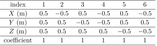
γ=45◦. In this experiment, a simulated target, instead of a real target, is used, as shown in Table 1.

The reason is that the true SCs of a real target are difficult to predict, which makes it hard to evaluate the result. Moreover, to make the analysis more clearly, the coefficient of each SC is supposed to be stable, and the shelter effect is not considered.

In Fig. 3, we give typical results with five different SNRs (25, 5, 0,−3, and−5 dB). The first column

presents the 1D SCs at different azimuth angles. As we can see, the 1D SCs produced by the same

3D SC are lined up. It should be noted that the 1D position, i.e., r_k(θ, γ), represents the projective

range along LOS of the k-th SC. According to Equation (2), when the elevation angle γ is constant,

the projective ranger_k(θ, γ) is a sinusoid over azimuth, which is in accordance with the performance in

Fig. 3. However, super-resolution algorithm produces some outliers. The proportions of outliers under different SNRs are listed in Table 2. We can see that the proportions of outliers grow with rising noise.

Table 1. A simulated target composed by eight scattering centers.

index 1 2 3 4 5 6

X (m) 0.5 −0.5 0.5 −0.5 0.5 −0.5

Y (m) 0.5 0.5 −0.5 −0.5 0.5 0.5

Z (m) 0.5 0.5 0.5 0.5 −0.5 −0.5

50 100 150 200 250 300 350 -2 -1.5 -1 -0.5 0 0.5 1 1.5 2

Azimuth(o)

R

a

nge(m

)

All points, HH channel

-2 -1 0 1 2 -2 -1 0 1 2 -2 -1 0 1 2

Real scattering centers Extracted scattering centers

50 100 150 200 250 300 350 -2 -1.5 -1 -0.5 0 0.5 1 1.5 2

Inliers, HH channel

Azimuth(o)

R

a

nge(m

)

(a)

50 100 150 200 250 300 350 -2 -1.5 -1 -0.5 0 0.5 1 1.5 2

Azimuth(o₎

R

a

nge(

m

)

All points, HH channel

-2 -1 0 1 2 -2 -1 0 1 2 -2 -1 0 1 2

Real scattering centers Extracted scattering centers

50 100 150 200 250 300 350 -2 -1.5 -1 -0.5 0 0.5 1 1.5 2

Inliers, HH channel

Azimuth(o₎

R a nge( m ) (b)

50 100 150 200 250 300 350 -2 -1.5 -1 -0.5 0 0.5 1 1.5 2

Azimuth(o₎

R

a

nge(

m

)

All points, HH channel

-2 -1 0 1 2 -2 -1 0 1 2 -2 -1 0 1 2

Real scattering centers Extracted scattering centers

50 100 150 200 250 300 350 -2 -1.5 -1 -0.5 0 0.5 1 1.5 2

Inliers, HH channel

Azimuth(o₎

R a nge( m ) (c)

50 100 150 200 250 300 350 -2 -1.5 -1 -0.5 0 0.5 1 1.5 2

Azimuth(o)

R

a

nge(

m

)

All points, HH channel

-2 -1 0 1 2 -2 -1 0 1 2 -2 -1 0 1 2

Real scattering centers Extracted scattering centers

50 100 150 200 250 300 350 -2 -1.5 -1 -0.5 0 0.5 1 1.5 2

Inliers, HH channel

Azimuth(o)

R a nge( m ) (d)

50 100 150 200 250 300 350 -2 -1.5 -1 -0.5 0 0.5 1 1.5 2

Azimuth(o₎

R

a

nge(

m

)

All points, HH channel

-2 -1 0 1 2 -2 -1 0 1 2 -2 -1 0 1 2

Real scattering centers Extracted scattering centers

50 100 150 200 250 300 350 -2 -1.5 -1 -0.5 0 0.5 1 1.5 2

Inliers, HH channel

Azimuth(o₎

R a nge( m ) (e)

Figure 3. Performance under different SNR conditions. (a) SNR = 25 dB. (b) SNR = 5 dB. (b)

Table 2. Proportions of outlier under different SNR conditions.

SNR(dB) 25 5 0 −3 −5

Proportion 1.67% 6.2% 20.42% 43.1% 56.67%

The second and third columns show the estimated 3D position of the SCs and their corresponding

inliers. In this experiment, we assume thatσ = 0.1, the maximum scope of the target is [−2 m, 2 m]×

[−2 m, 2 m]×[−2 m, 2 m] andN = 20000. Using the parameters mentioned above, the tolerance εcan

be calculated as 0.0375 m. The maximum number of points at each aspect is 6, thus a 4×30 matrix is

used for the multiple model storage. By comparing the results, we note that the model can be extracted

correctly when SNR is−3 dB or higher, while fraction of outliers is up to 43.1%. The results show that

the proposed methodology is robust to tolerate a tremendous fraction of outliers.

4.2. The Validity of the Extracted SCs

The scattering coefficient of a SC varies smoothly with aspect. It is a very important characteristic in checking the validity of the result. For example, when two SCs are considered as one, the scattering coefficient of the integrated SC is obtained by summing up the contributions from two SCs. Since the phases of the two SCs are sensitive to LOS, the integrated scattering coefficient varies roughly with aspects. In the extreme case, when all SCs are combined into one, the integrated scattering coefficient actually is the conventional radar cross section. Another useful characteristic is that the SCs are not particular to radar system parameters such as the operating frequency, bandwidth and waveform. Therefore, once the SCs are obtained by given wide-band measurements, the data in adjacent frequency-band are available. Moreover, the performances of the constructed data are consistent with that of measured data in practice, such as the RCS, high range resolution profile (HRRP), ISAR image, etc.

In order to illustrate the validity of the SCs, we take a cone-shaped target as an example, as shown in Fig. 4. The center frequency is 10 GHz. The bandwidth is 4 GHz, and the number of slant-range bins

is 200. Fig. 5 shows the schematic of the experimental setup. The azimuth angleθvaries from−90◦ to

90◦ with angle interval 0.2◦. In order to prove the robustness of the model, we extract the SCs using

the measurements in 8–10 GHz and validate them using the measurements in 10–12 GHz.

Figure 4. Geometry of the cone-shaped target.

x

y

o -90

o 0

o 90

Figure 5. The schematic of the experimental setup.

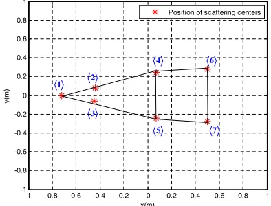
By performing the proposed methodology, seven SCs are obtained, as shown in Fig. 6, where we

mark them as 1,2,. . .,7. The contour of the target is also depicted. One can see that the model

-1 -0.8 -0.6 -0.4 -0.2 0 0.2 0.4 0.6 0.8 1 -1

-0.8 -0.6 -0.4 -0.2 0 0.2 0.4 0.6 0.8 1

x(m)

y(

m

)

Position of scattering centers

1 2

3

4

5

6

7

Figure 6. The position of SCs obtained by the proposed methodology.

-100 -80 -60 -40 -20 0 20 40 60 80 100

-100 -80 -60 -40 -20 0 20 40 60 80

Azimuth(o₎

RCS

(d

B

)

scattering coefficient of scattering center <1> scattering coefficient synthesized by <1>,<2> and <3>

Figure 7. The scattering coefficient of 1 and

the synthesized SC composed by1,2and3.

-100 -80 -60 -40 -20 0 20 40 60 80 100

-120 -100 -80 -60 -40 -20 0 20 40 60

Azimuth(o₎

RCS(

d

B

)

Reconstructed data Measured data

0 20 40 60 80 100 120

0.1 0.2 0.3 0.4 0.5 0.6 0.7 0.8 0.9 1

Number of range cell

N

o

rm

a

liz

ed

amp

lit

ude

Reconstructed data Measured data

(b) (a)

Figure 8. Comparison between measured data and simulated data in 10–12 GHz. (a) RCS data. (b) HRRP.

coefficient of SC1is shown in Fig. 7. It is noted that scattering coefficient varies smoothly from−40◦

to 40◦. However, in other aspects, the scattering coefficient may change roughly. The reason is that the

response of SC is an approximation to the real responses from a small region on the target. In some aspects, the error produced by the approximation may occur, yielding to an aspect-sensitive coefficient

at these aspects. In all, the scattering coefficient of 1 is stabile in a broad angular extent, which

demonstrates the effectiveness of the result. On the other hand, when1,2 and3 are extracted as

one synthesized SC, the scattering coefficient of the synthesized scattering center is expressed as a green

line with ‘+’ marker. Compared with1, one can see that the scattering coefficient of the synthesized

one changes roughly almost at all aspects, which behaves in accordance with what’s mentioned above. In order to evaluate the robustness of the SCs, the wide-band data measured in 10–12 GHz are compared with the data in the same frequency-band simulated by the model. Fig. 8(a) shows the RCS data reconstructed by these two kinds of data, where the parameters used in calculating the simulated RCS data are supposed to be the same as original measurements. As we can see, the RCS data are

approximately the same at different azimuth angles. In the case of θ=16◦, the HRRPs of the two data

are shown in Fig. 8(b), from which one can find that the locations and amplitudes of the peaks in the HRRP are in accordance with each other.

Furthermore, Fig. 9 shows ISAR images obtained by the data measured in 8–12 GHz, constructed

Number of range cell

N

u

m

b

er of

c

ros

s

-ra

ng

e c

e

ll

60 80 100 120 140 160 180 60

80

100

120

140

160

180

Number of range cell

N

u

m

b

er

of

c

ros

s

-range

c

e

ll

60 80 100 120 140 160 180 60

80

100

120

140

160

180

Number of range cell

N

u

m

b

er

of

c

ros

s

-range

c

e

ll

60 80 100 120 140 160 180 60

80

100

120

140

160

180

(a) (b) (c)

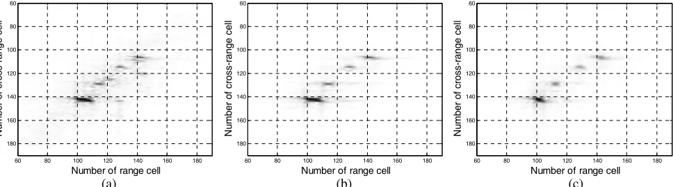
Figure 9. ISAR images obtained by different data. (a) The data measured in 8–12 GHz. (b) The data simulated in 8–10 GHz. (c) The data simulated in 10–12 GHz.

synchronized aperture is 12.8◦ with 0.2◦ sampling interval. As we can see, the location and amplitude

of most of the peaks in the original image are retained in the reconstructed ones. Thus, the results have demonstrated the effectiveness of the extracted SCs.

5. EXPERIMENTAL RESULTS

In this section, we make use the electromagnetic simulated data of a ship target to demonstrate the practical importance of this work. First, the performance is evaluated to verify the effectiveness of the proposed methodology. After that, we investigate the validity of the SCs at adjacent elevation angles.

5.1. Performance Evaluation

The geometry of the ship model is illustrated in Fig. 10. The length, width, and height of the target are 173 m, 16.8 m, 51 m, respectively. The original data are produced by electromagnetic simulation. The frequency is sampled from 16.975 GHz to 17.025 GHz with 151 sample points. The bandwidth is 50 MHz, which means that the range resolution is 3 m. It should be noted that the bandwidth in this experiment is much smaller than other examples. The reason is that the size of a ship is much larger than the targets in other examples. The range resolution of 3 m is sufficient to illustrate the target radar signature. Moreover, if we expand the bandwidth to 500 MHz with the same frequency step, several

months will be needed for data collection. The elevation is 30◦, while the azimuth varies from 0◦ to

360◦ with angle interval 1◦, thus we haveN = 360.

In [13], local 2D SCs are used in the 3D SC extraction where the 2D SCs are extracted via the data collected in a small aperture. Suppose that the data are obtained at a series of stepped azimuth

angles {Δθ 2Δθ . . . vΔθ . . . VΔθ}, where Δθ and V denote the angle step and total number of

sampling points in azimuth, respectively. Then the phase of a SC on the target can be expressed as

φSC(v) = 2π2r_λSC sinvΔθ (9)

whereλis the wave length andr_SCthe distance to the rotational centre along the cross range. Generally,

the aperture is small enough that the approximation holds:

sinvΔθ≈vΔθ. (10)

Then Equation (7) can be rewritten as

φSC(v) = 2π2rSCΔθ

λ v. (11)

According to Nyquist sampling theorem, to avoid the overlapping effect, the coefficient of v should be

smaller than 2π, i.e.,

2π2rSCΔθ

λ <2π ⇒ Δθ < 2rλ_SC . (12)

The distancer_SC is smaller than 173 m. Using the parameters mentioned above, Equation (12) can be

rewritten as Δθ <0.0029◦. This angle step is too small to be feasible.

For our methodology, we assume the maximum scope of the target [−150 m,150 m]×[−50 m,50 m]×

[−50 m,50 m], threshold value σ = 5 m and maximum iterations N = 500000, respectively. The

maximum number of points at each aspect is 10, thus a 4×100 matrix is used for the multiple model

storage. In Step B-5, the tolerance ε can be calculated as 1.5 m. In Step B-8, we suppose that the

predefined fraction Γ is 65%, and 20 SCs are obtained.

Using a Pentium 4 3.0 GHz CPU and MATLAB Ver. 7.1, the average computation time for the proposed method is 1143 s. Fig. 11(a) shows all points in data obtained by 1D SC estimation at different azimuths. Fig. 11(b) shows the inliers which correspond to the extracted 3D SCs. It is obvious that the outliers are scattered about the inliers, which are lined up in this figure. After taking the proposed methodology, most of the outliers are removed, which shows the robustness to tolerate the outliers. The extracted 3D SCs are shown in Fig. 12. In order to exhibit the distribution of SCs more clearly, the results are positioned in the same Cartesian coordinates as the CAD model. As we can see, most SCs are in accordance with the target structure, and most of them are located on the tips or edges on the target surface, while one SC is apart from the target. We think that it may result from multipath or produced by the outliers in 3D position estimation.

In order to validate the effectiveness of the proposed procedure, the reconstructed RCS of different frequencies, reconstructed HRRP, and reconstructed RCS of different azimuth angles are used to evaluate the estimation results. Figs. 13(a) and 13(b) depict the RCSs of different frequencies and HRRPs

obtained atθ= 311◦, while Figs. 13(c) presents the RCSs of different azimuths. As we can see, the RCS

data behave approximately the same at different frequencies and azimuths; the locations and amplitudes

50 100 150 200 250 300 350

-100 -80 -60 -40 -20 0 20 40 60 80 100

Azimuth(o₎

R

ange(m

)

Elevation 30o _{, HH channel, All points}

50 100 150 200 250 300 350

-100 -80 -60 -40 -20 0 20 40 60 80 100

Elevation 30o _{, HH channel, Inliers}

Azimuth(o₎

R

ange(m

)

(a) (b)

Figure 12. The position of the extracted SCs in the CAD model.

1.6975 1.698 1.6985 1.699 1.6995 1.7 1.7005 1.701 1.7015 1.702 1.7025 x 1010

5 10 15 20 25 30 35 40 45 50

Frequency(Hz)

A

m

pl

it

ude(dB

)

Azimuth 311o_{, Elevation 30}o _{, HH channel}

Original RCS Constructed RCS

-150 -100 -50 0 50 100 150 10

20 30 40 50 60 70

Range(m)

A

m

plitude(

dB

)

Azimuth 311o_{, Elevation 30}o _{, HH channel}

Original HRRP Constructed HRRP

0 50 100 150 200 250 300 350 400 10

15 20 25 30 35 40 45 50

Azimuth angle(o₎

RCS(

d

B)

Frequency 16.975GHz ,Elevation 30o _{, HH channel}

Original RCS Constructed RCS

(a) (b) (c)

Figure 13. Comparison of the two methods. (a) Reconstructed RCS of different frequency. (b) HRRP. (c) RCS of different azimuth angle.

Azimuth angle(o₎

R

a

nge(

m

)

Original,Elevation 30o _{, HH channel}

50 100 150 200 250 300 350

-150

-100

-50

0

50

100

150 -1

-0.5 0 0.5 1 1.5 2 2.5 3 3.5 4

Azimuth angle(o₎

R

a

nge(

m

)

Reconstruct,Elevation 30o _{, HH channel}

50 100 150 200 250 300 350

-150

-100

-50

0

50

100

150

-1 -0.5 0 0.5 1 1.5 2 2.5 3 3.5 4

(a) (b)

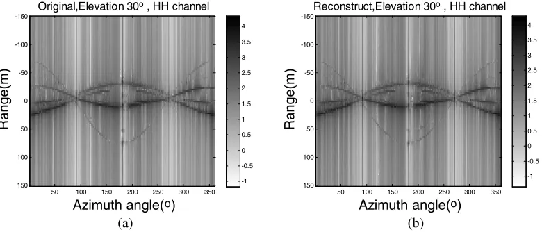
Figure 14. Comparison of range profiles at all azimuth angles. (a) Original data. (b) Reconstructed data.

of the peaks in the original range profile can be retained in the reconstructed range profile as well. In order to evaluate the performance of the SCs at different azimuths, the range profiles at all azimuths are given in Fig. 14, where the gray level of the pixels corresponds to the logarithm amplitude of the range profiles. One can see that a few dark curves crossing different angular extents in the original figure, which implies the regular variation in projective locations of the stable SCs. By comparing the results, we see that the intensity and locations of the dominant SCs are retained in the reconstructed profiles at all azimuths.

coefficient and HRRP correlation coefficient. They can be defined as follows, respectively.

Correlation_RCS= 1

MN M m=1 N n=1 H h=1

|rcs(h)rcs_simu(h)|2

H

h=1

|rcs(h)|2

L

l=1

|rcssimu(h)|2

(13)

Correlation_HRRP= 1

MN M m=1 N n=1 S s=1

|hrrp(s)hrrp_simu(s)|2

S

s=1

|hrrp(s)|2

S

s=1

|hrrpsimu(s)|2

(14)

where rcs(h) denotes the original RCS measured at different frequencies; h = 1,2, . . . , H is the

frequency-sampling points; rcs_simu(h) is the reconstructed RCS; hrrp(s) and hrrp_simu(s) are the

constructed range profile and original range profile, respectively; s = 1,2, . . . , S is the index of the

range bin. The correlation coefficients are listed in Table 3, which demonstrates the effectiveness of this methodology.

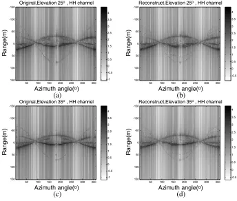
5.2. Validity of the SCs at Adjacent Elevation Angles

The 3D SCs in this paper are extracted using the data at a single elevation. However, we advocate its applicability in a large angular extent. In this section, we predict the wide measurements and HRRPs

Azimuth angle(o₎

R

a

nge(

m

)

Original,Elevation 25o _{, HH channel}

50 100 150 200 250 300 350 -150 -100 -50 0 50 100 150 -1 -0.5 0 0.5 1 1.5 2 2.5 3 3.5 4

Azimuth angle(o₎

R

a

nge(

m

)

Reconstruct,Elevation 25o _{, HH channel}

50 100 150 200 250 300 350 -150 -100 -50 0 50 100 150 -0.5 0 0.5 1 1.5 2 2.5 3 3.5 4 (a)

Azimuth angle(o)

R

a

nge(

m

)

Original,Elevation 35o _{, HH channel}

50 100 150 200 250 300 350 -150 -100 -50 0 50 100 150 -1 -0.5 0 0.5 1 1.5 2 2.5 3 3.5 4

Azimuth angle(o)

R

a

nge(

m

)

Reconstruct,Elevation 35o _{, HH channel}

50 100 150 200 250 300 350 -150 -100 -50 0 50 100 150 -0.5 0 0.5 1 1.5 2 2.5 3 3.5 4 (c) (b) (d)

Figure 15. Comparison of range profiles at all azimuth angles. (a) Original data under elevation

γ = 25◦. (b) Reconstructed data under elevation γ = 25◦. (c) Original data under elevation γ = 35◦.

Table 3. Correlation coefficients of the two methods.

Correlation coefficients Proposed method

Correlation_RCS 0.9632

Correlation_HRRP 0.9713

at other elevations via the 3D SCs, which are obtained by the proposed methodology, then evaluate the validity of the SCs at adjacent elevation angles by comparing them with that calculated by the high frequency electromagnetic simulation software.

Since the scattering coefficient varies smoothly with aspect, we suppose that the scattering

coefficient of a SC under elevation angle γ=35◦ or 25◦ approximates to that of γ=30◦. Thus the wide

measurements under elevation angle γ=35◦ or 25◦ can be obtained according to Equation (1). Fig. 15

compares the range profiles at all azimuths using different data. The first and second rows correspond

to elevation γ=25◦ and elevation γ=35◦, respectively. The first column shows the range profiles using

the original data while the second column is generated by the reconstructed data obtained via Equation

(1). According to Equation (14), the HRRP correlation coefficients are Correlation_HRRP = 0.843 and

Correlation_HRRP = 0.888 under elevation angleγ=35◦ and 25◦, respectively. The results show that the

SCs are valid at adjacent elevation angles, which demonstrate the practical importance of the proposed methodology.

6. CONCLUSIONS

The 3D SC model is very useful for target recognition and data compression. However, the existing methods are difficult to be accomplished for high frequency signal or large-size target. The reason is that the dense sampling in azimuth is hard to achieve. To solve this problem, a new methodology is proposed in this paper. The 1D SCs extracted at different aspects are applied to extract 3D SCs, where the outliers induced by 1D SC estimation are resolved by a modified RANSAC method. Moreover, the discretization of the parameter space in [13] is unnecessary, which means that the proposed methodology does not suffer from limited accuracy. Experiments demonstrate the effectiveness of the proposed approach.

ACKNOWLEDGMENT

This work was supported by the National Natural Science Foundation of China (Grant No. 61401479).

REFERENCES

1. Keller, J. B., “Geometrical theory of diffraction,” J. Opt. Soc. Amer, Vol. 52, No. 2, 116–130, Feb.

1962.

2. Potter, L. C., D. M. Chiang, R. Carriere, and M. J. Gerry, “A GTD-based parametric model for

radar scattering,” IEEE Trans. Antennas Propag., Vol. 43, No. 5, 1058–1067, Oct. 1995.

3. Hurst, M. P. and R. Mittra, “Scattering center analysis via Prony’s method,” IEEE Trans.

Antennas Propag., Vol. 35, No. 5, 986–988, Aug. 1987.

4. Potter, L. C. and R. L. Moses, “Attributed scattering centers for SAR ATR,”IEEE Trans. Image

Process., Vol. 6, No. 1, 79–91, Jan. 1997.

5. Bhalla, R., J. Moore, and H. Ling, “A global scattering center representation of complex targets

using the shooting and bouncing ray technique,” IEEE Trans. Antennas Propag., Vol. 45, No. 5,

1850–1856, Dec. 1997.

6. Zhou, J., H. Zhao, Z. Shi, and Q. Fu, “Global scattering center model extraction of radar targets

based on wideband measurements,” IEEE Trans. Antennas Propag., Vol. 56, No. 7, 2051–2060,

7. Zhai, Q. L., W. Wang, J. M. Hu, and J. Zhang, “Azimuth nonlinear chirp scaling integrated with

range chirp scaling algorithm for highly squinted SAR imaging,” Progress In Electromagnetics

Research, Vol. 143, 165–185, 2013.

8. Hu, J. M., W. Zhou, Y. W. Fu, X. Li, and N. Jing, “Uniform rotational motion compensation for

ISAR based on phase cancellation,” IEEE Geosci. Remote Sensing Lett., Vol. 8, No. 4, 636–640,

Jul. 2011.

9. Hu, J. M., J. Zhang, Q. L. Zhai, R. H. Zhan, and D. W. Lu, “ISAR imaging using a new

stepped-frequency signal format,”IEEE Trans. Geosci. Remote Sens., Vol. 52, No. 7, 4291–4305, Jul. 2014.

10. Margarit, G., J. J. Mallorqu´ı, and X. F`abregas, “Single-pass polarimetric SAR interferometry for

vessel classification,” IEEE Trans. Geosci. Remote Sens., Vol. 45, No. 11, 3494–3502, Nov. 2007.

11. Margarit, G., J. J. Mallorqui, J. Fortuny-Guasch, and C. Lopez-Martinez, “Exploitation of ship

scattering in polarimetric SAR for an improved classification under high clutter conditions,”IEEE

Trans. Geosci. Remote Sens., Vol. 47, No. 4, 1224–1235, Apr. 2009.

12. Zhang, J., J. Hu, Y. Gao, R. Zhan, and Q. Zhai, “Three-dimensional scattering centers extraction of

radar targets using high resolution techniques,”Progress In Electromagnetics Research M, Vol. 37,

127–137, 2014.

13. Zhou, J., Z. Shi, and Q. Fu, “Three-dimensional scattering center extraction based on wide aperture

data at a single elevation” IEEE Trans. Geosci. Remote Sens., Vol. 53, No. 3, 1638–1655, Mar.

2015.

14. Fisher, M. and R. Bolles, “Random sample consensus: A paradigm for model fitting with

applications to image analysis and automated cartography” Comm. of the ACM, Vol. 24, No. 6,

381–395, 1981.

15. Kim, T. J. and Y. J Im, “Automatic satellite image registration by combination of matching and

random sample consensus,” IEEE Trans. Geosci. Remote Sens., Vol. 41, No. 5, 1111–1117, May

2003.

16. Chum, O. and J. Matas, “Optimal randomized RANSAC,”IEEE Transactions on Pattern Analysis

and Machine Intelligence, Vol. 30, No. 8, 1472–1482, Aug. 2008.

17. Roy, R. and T. Kailath, “ESPRIT-estimation of signal parameters via rotational invariance

techniques,”IEEE Trans. on Acoust. Speech. Signal Processing, Vol. 37, No. 7, 984–995, Jul. 1989.

18. Stoica, P. and A. Nehorai, “MUSIC, maximum likelihood, and Cramer-Rao bound,”IEEE Trans.

on Acoust. Speech. Signal Processing, Vol. 37, No. 5, 720–741, May 1989.

19. Huffel, S. V., H. Park, and J. B. Rosen, “Formulation and solution of structured total least norm

problems for parameter estimation”IEEE Trans. Signal Process., Vol. 44, No. 5, 2464–2474, Oct.

1996.

20. Hua, Y. and T. K. Sarkar, “Matrix pencil method for estimating parameters of exponentially

damped/undamped sinusoids in noise,” IEEE Trans on Acoust. Speech. Signal Processing, Vol. 38,

No. 5, 814–824, Aug. 1987.

21. Yan, X. W., J. M Hu, G Zhao, J. Zhang, and J. W. Wan, “A new parameter estimation method

for GTD model based on modified compressed sensing,” Progress In Electromagnetic Research,

Vol. 141, 553–575, 2013.

22. Dai, D. H., X. S. Wang, Y. L. Chang, J. H. Yang, and S. P. Xiao, “Fully-polarized scattering center

extraction and parameter estimation: P-SPRIT algorithm,” Proc. Int. Conf. Radar, CIE 2006,