OTTO JOHNSTON
ABSTRACT. We give an improved index calculus attack for a large class of elliptic curves. Our algorithm works by efficiently transferring the group structure of an elliptic curve to a weaker group. The running time of our attack poses a significant and realistic threat to the security of the elliptic curves in this class. As a consequence of our construction, we will also derive entirely new point counting algorithms. These algorithms set new run-time complexity records. We discuss implementations of these algorithms and give examples.
1. INTRODUCTION
A discrete logarithm problem for a groupGsimply asks for the computation ofxin a pair(g, gx) forg ∈ G. In most cases, we wantGto be efficiently representable, finite, andalmostof prime order. This almost of prime order property means that G should contain a large prime order subgroup relative to its size. Such a subgroup is necessarily cyclic, and if G is very large, then efficiently computing discrete logarithm instances cannot be accomplished by using general finite group theory (e.g., Sylow’s theorems, Chinese Remainder Theorem).
On a high level, what we look at is the case where we have another groupH and a surjective homomorphism
f : H → G. In this case, there exists an h ∈ H such that f(h) = g and consequentlyf(hx) = gx. Thus, computing x for a pair (h, hx) is at least as difficult as computing it for (g, gx) provided that the difficulty of computingf−1 does not get in the way. In the case of elliptic curve cryptography, the groupGis replaced by an elliptic curveE. Only the group structure of this curve is important, so one can think ofE as a new letter for the groupG. The groupEis always efficiently representable and finite, and it is sampled so that it is almost of prime order. Most importantly, the computation of discrete logarithm problems onE is a notoriously difficult problem that has resisted decades of attacks. What we show in this paper is how to efficiently construct a new groupHsuch that there is a surjective homomorphismH →Ewith an efficiently computable inverse. We then show how to use the structure ofHto make it easier to compute discrete logarithms for a large family of elliptic curves.
1.1. Historical Overview of Index Calculus Attacks on Elliptic Curves. We now give a brief historical overview of the results we will need. Since elliptic curves are centuries old and the central topic of numerous papers each year, our overview is far from complete. See [33] for a more complete survey. For general elliptic curves, the best known algorithm to compute discrete logarithms is the Pollard-Rho algorithm, which computes the discrete logarithms of a groupG in time equal toO(√p), where pis the largest prime factor of #G. There have been numerous efforts to do better than this whenGis an elliptic curve. J. Silverman in [34] was the first to propose an index calculus variant for elliptic curves that was hoped to have a faster running time than Pollard-Rho. Very shortly thereafter, this approach was shown to be slower (see [17]). Roughly a decade earlier, N. Koblitz had proposed a generalization of elliptic curve cryptography to hyperelliptic curves in [21]. This system was brought into question by P. Gaudry in [14], where it was shown that index calculus for hyperelliptic curves worked with a remarkable advantage: in [14], he was able to run his algorithm to calculate a challenge discrete logarithm problem using only modest hardware. Once P. Gaudry proposed his attack against hyperelliptic curves, many generalizations quickly followed (see [7], [9], [16], [35]).
Although Gaudry’s methods did not seem to have any direct advantage when used for elliptic curves, an attack against elliptic curves surfaced anyway. The idea was totransferthe group structure of an elliptic curve to one of the weaker hyperelliptic curves. The idea goes as follows. The running time of the generic discrete logarithm attacks against an elliptic curve overFqis roughlyO(
√
q), whereas the running time of index calculus on a hyperelliptic curve over the same field is roughlyO(q2−2/g)forg ≥2. This second attack does not help at all, unless we had a situation where the elliptic curve, call itE, was defined overFqnand the hyperelliptic curve, call itC, was defined over the subfieldFq. If the group structures related toE andC were isomorphic and ifn > 2, we could gain a
Date: November 11th, 2010.
computional advantage by using index calculus on the hyperelliptic curve if we could compute this isomorphism in reasonable time. This is the basic idea behind the so-calleddescenttheory of index calculus on elliptic curves. This descent procedure stimulated a great deal of investigation (see [12]) and resulted in a remarkable reduction in the security of many elliptic curves over even extensions of finite fields in characteristic2. However, in odd characteristic, this attack was more difficult.
1.2. The mathematics behind the descent of index calculus. The main difficulty in transferring a discrete log-arithm problem from an elliptic curve to a higher genus curve is at the heart of a very deep problem in algebraic geometry. From a computational point of view, whether one is interested in point counts or cryptographic applica-tions, a curve serves as a platform to construct an object known as a Jacobian. The Jacobian is the real object of interest in virtually any application point of view; the curve merely serves as a method to construct it. A Jacobian lives in a more general class of objects known as abelian varieties. A very difficult and fundamental problem in algebraic geometry is to understand the interplay between the Jacobians and the abelian varieties that are not Ja-cobians, and, most importantly for us, a deep problem asks about surjective homomorphisms with small kernels between these objects.
The surjective homomorphisms we are looking for most naturally come from the theory of isogenies. An isogeny is a morphism between abelian varieties that is both surjective and has a finite kernel. These maps give us more freedom in trying to deform the elliptic curve into the Jacobian of a higher genus curve without destroying the underlying discrete logarithm problem. In particular, if an isogenyf : A → B has a kernel in some part ofA
that is small, say a few elements of order2, then one could hope that by studying f one could transfer discrete logarithms with more freedom than if we restricted to isomorphisms. In geometric language, we would be studying the so-called isogeny classes.
1.3. Our results. The theoretical contributions of this article are two-fold. The first is a technical result: we prove that under a certain condition, ifAis an abelian variety that is isogenous to the Jacobian of a hyperelliptic curve, then so isA2. The second contribution is that these constructions are computationally efficient. These two results are then applied to two extremely active problems in computational algebraic geometry: the computation of discrete logarithms on elliptic curves and point counting algorithms for hyperelliptic curves.
1.3.1. Implications to cryptographic schemes. The main contribution of this paper is to give the first new class of ordinary elliptic curves where index calculus becomes a practical threat. We will show how to sample from this family efficiently. We require no extra side information to apply our attack, nor do we need special oracles or structure information about the elliptic curves we sample. Moreover, every member of the family we create will be vulnerable to our descent attack. We show how to use this construction to build a large and explicit family of elliptic curves where a factor basis for index calculus can be found and used to compute discrete logarithms in time roughlyO(q3/8), where the generic attacks on the same curve would run in time roughlyO(q1/2).
The implications to actual in-use schemes are the following. There are three ways for a given security parameter
k∈Z+to influence the group size of a family of elliptic curves. The first is to usekas the bit-length of a primep and define elliptic curves overFp, the second is to fixpand define elliptic curves overFpk, and the third is some combination of the first two. It was previously known that if we tookp= 2andk >2to be a power of2that there were elliptic curves overF2k that were weak in the sense described above (see [12]). We extend this result to all primesp. Our results show that elliptic curve cryptography must take special care whenkis taken as an exponent ofanyfixed prime or ifkinfluences both the prime size and its exponent. Both of these statements are new.
The explicit family of weak elliptic curves we will construct contains instances of virtually all elliptic curve classes proposed in the literature. Most importantly, if we sample random curves from this family, we find elliptic curves with large prime factors that have not been previously ruled out as cryptographically weak. We will give examples of elliptic curves with a group size in the 160 bit range with a single large prime factor that can be attacked with a substantial advantage over the generic algorithms.
had a surjective map (with a small kernel) to a curveE0 that did satisfy this special property, thenE would be as vulnerable asE0 to the attack we outline in this paper. There is computational evidence that an enormous increase in the number of weak curves might be found in this way, but due to the incomplete picture of how elliptic curve families are distributed among their associated groups, we cannot offer any proofs.
1.3.2. Point Counting. A very difficult problem in computational algebraic geometry is to generate large families of curves with a known number of points over a finite fieldFq. The parameters one usually wants to consider are
qand an invariant of the curve known as its genus. One should view the genusgand the numberqas integers that specify intrinsic properties ofC. In order to hope for efficient computations of the number of points ofC, one must restrict the class of curve in some way.
The current state of the art algorithm for generating genus 2 curves with a known number of points is that given by Satoh in [30]. Satoh’s algorithm works by taking two isomorphic elliptic curves and glueing a genus2
curve from these equations. Relaxing the condition of isomorphism to that of isogeny, we are able to make a new algorithm for this purpose. Our algorithm is superior to Satoh’s in the following ways. (1) It outputs the group order rather than merely the largest prime factor. (2) It outputs the group orderwith certainty, rather than merely with some probability that is not well-understood. (3) It allows for a much wider distribution of curves, in contrast to Satoh’s algorithm which is restricted to even orders. In particular, our algorithm can be used to find prime-order Jacobians. We also drastically reduce the complexity of Satoh’s algorithm fromO(log2(q))operations overFqto
O(log(q))overFq.
We are also able to propose entirely new point counting algorithms based on this work. One such extension is an algorithm that generates genus 4 curves along with the order of their Jacobian at the cost of running a point counting algorithm on a single elliptic curve. This algorithm is a significant improvement over existing point counting algorithms (see [29]). In fact, we will be able to compute the entire Zeta function for the genus4curve, which essentially classifies the genus4curve’s arithmetic properties.
As a final application to point counts, we will show how to generate a large class of hyperelliptic curves of genus
2goverFqwith exactlyq+ 1points inO(glog(q))operations overFq. To generate these curves, we only require a positive integerg and an odd prime powerq as an input to our algorithm. This algorithm remains efficient ifg
grows linearly andqgrows exponentially, which is unlike any previous curve generation algorithm for a family as large as the one we will consider (for previous work, see [29], [19]).
1.4. Organization. In the next section, we will collect the results we need at a high level to run our attack. We will then proceed to prove them in detail. In Section 3, we will write out our point counting algorithms using the material in Section 2. In Section 4, we give an algorithm that efficiently computes the transfer map explained earlier in this introduction and we outline the discrete logarithm attack. In Section 5, we discuss the distributions of the elliptic curves we sample. We conclude with a link to implementations of our algorithms.
2. ADESCENT OF HYPERELLIPTIC CURVES
2.1. An outline. Before we begin with a formal discussion, we will give an outline of what we prove and how we use it. We will first fix a finite fieldk0 in odd characteristic. In this discussion, we have two objects. The first are hyperelliptic curves. On the level of equations, a hyperelliptic curve is given by a formula of the formy2 =f(x), wheref is a separable polynomial in the variable x. The second class of objects we deal with are Jacobians of hyperelliptic curves. These objects can be thought of as unpacking the “group structure” of the equation forC. For instance, in elliptic or hyperelliptic curve cryptography, the curve serves only as a means to efficiently represent the group structure of its Jacobian. It is in this group that all of the calculations are done. In coding theory, this unpacking procedure is used to construct vector spaces with interesting parameters.
In our setting, we will letk be a quadratic extension ofk0. It is well known that kcan be formed by taking the square root of a non-square ink0, and we will letwbe this square root. If we letC be the hyperelliptic curve defined by
y2= (x−w)f(x),
we can show that there is another hyperelliptic curveC0of the form
defined overk0. The curveC0has the special property that the Jacobian ofChas a homomorphism to the Jacobian ofC0 on the level of groups. This map, call itδ, is almost an isomorphism: in Theorem 2, we show that it is an isomorphism modulo points of order2. Another critical property is thatδis computationally efficient to compute. These two results give us a descent. We are able to construct thisC0 from Theorem 1, and we can read off the polynomialg(x)above from Corollary 1.
The mapδis almost all we need for the discrete logarithm attack. To make the attack practical, we also need to know the order of the Jacobian ofC0. This takes a little more effort, but Corollary 3 gives us this order. Our strategy is to then find elliptic curvesEand to build the curvesC0. Once we haveC0, we try to apply the descent again. If we can descend once more, we then have a computationally efficient map fromE to the Jacobian of a genus4hyperelliptic curve. Since index calculus works with a remarkable advantage with these curves (see [35]), we have successfully attackedE.
2.2. The mathematics behind the descent. We will now proceed to prove these ideas, but as we move toward the details we are forced to become more precise. We will letkbe a finite field in odd characteristic. By acurve overk, we will mean a projective, geometrically irreducible variety of dimension 1 overkthat has at least one non-singular rational point. We do not assume our curves are non-singular. Given a curveC, we will letCedenote the normalization ofC, and we will let any arrowCe → C reference the implicit normalization map whenever it is needed. For a curveC, we will let Jac(C) denote the Jacobian ofCe. When a curve is specified by an affine equation, we will always take the projective closure. Ahyperelliptic curveis a curve that admits a double covering of a conic.
Our first task is to glue two hyperelliptic curves to produce a new curve. Although this is a classical result, we will reprove it with an emphasis on deriving an affine equation for the new curve. In the next series of proofs, we will continue to keep track of equations. Eventually, this will lead us to the new algorithms in the later sections. We will assume that all of our fields are finite fields, even though many of these results are more general.
Lemma 1. LetC1 : y2 = f and C2 : y2 = g be two hyperelliptic curves defined over k, wheref andg are separable polynomials ink[x]withh=f g/(gcd(f, g))2∈/ k. If we letC3 :y2=h, then the curve
(2.1) C:y4= 2(f +g)y2−(f−g)2
has the property that
Jac(C)∼ 3 Y
i=1
Jac(Ci).
Proof. In order forC to have a function field, it must be geometrically irreducible; by inspecting the roots of the
equation forC ink(x)[y], we see that this implies that√f gis not ink(x), which is whereh /∈kis used. Let the function field ofC1bek(x)[y1]and let the function field ofC2bek(x)[y2]. If we take the compositum,k(x)[y1, y2], theny = y1+y2 is permuted by the Galois actions of Gal(k(x)[y1]/k(x)) = {1, ψ}and Gal(k(x)[y2]/k(x)) = {1, φ}. This implies thatk(x)[y1, y2] = k(x)[y]. It is easy to see that the minimal polynomial Irrk(x)(y) is the equation forCgiven above: it is simplyQ
(y±(y1±y2)). Now, Gal(k(x)[y]/k(x)) =Z/2Z×Z/2Z, and it is
obvious thatC/ψ ∼=C2,C/φ∼=C1, andC/(ψφ)∼=C3. We apply Theorem5of [18] to obtain thek-isogeny Jac(C)∼YJac(Ci).
We will construct a new hyperelliptic curve that captures the arithmetic data of a smaller genus hyperelliptic curve. Our new hyperelliptic curve will be defined over a smaller field, and it is from here where our descent from smaller genus curves to larger genus curves begins.
LetC be any curve overk and letk/k0 be a finite extension. GiveC an affine equationP
i,jci,jxiyj = 0as before, where only theci,j are ink. For any automorphismσ∈Aut(k/k0), letσ(C)denote the smooth, projective curve with affine equationP
i,jσ(ci,j)xiyj. In order for us to allowσ to act on points ofC, we need to work in a larger ambient space. To extendσ, associate each closed pointP ∈P2
denote the forgetful functorΓ :AbSch/k→Ab from the category of abelian group schemes overkto the category of abelian groups: it simply takes an abelian group scheme to its underlying group.
Lemma 2. IfCis any curve defined overksuch that there exists a subfieldk0 ⊂k, then for anyσ ∈Gal(k/k0), we have Jac(C)∼Jac(σ(C)). Moreover,σextends to an isomorphismΓ(Jac(C))∼= Γ(Jac(σ(C))).
Proof. For any finite extensionk⊂l, if we have anl-rational pointPofC, thenσ(P)is anl-rational point ofσ(C)
by definition. Thus,σestablishes a bijection between the rational points ofCandσ(C)over any finite extension of
k. This implies that they have the same Zeta function and hence the sameL-polynomial. Since theL-polynomial classifies an isogeny class (see Theorem 2.c, Appendix 1, [27]), our result follows.
Any divisorial correspondenceD∼D0 comes from a rational functionf ∈k(C). If we writeD=P
Piand letσ(D)denoteP
σ(Pi), we see at once thatσ(D)∼σ(D0)viaσ(f), where, again,σ(f)is simplyσ applied to the coefficients off ink. Clearly, composingσwithσ−1gives us the identity; since it is obviously homomorphic,
we have an isomorphismΓ(Jac(C))∼= Γ(Jac(σ(C))).
Example 1. The map σ above is not typically in the image of the Picard functor. In other words, Jac(C) and Jac(σ(C))are not usually isomorphic as varieties. It is this key property that gives us a very large distribution to sample from, and it is one of the main features where our approach differs from other work. Essentially, we have two Jacobians that are isomorphic as abelian groups but not as varieties. To make sense out of what this means, some examples are in order. Consider the finite fieldk=F5[w], wherew2= 2. Define the elliptic curve
E1 :y2= (x−w)(x2−x). By our construction (k0=F5andσbeing absolute Frobenius),
E2 =σ(E1) :y2 = (x+w)(x2−x).
The previous result might lead one to think that the Pic0functor is represented by the same abelian group scheme for both curves, and hence isomorphic (by the universal property of representability). This would indeed be the case ifσ was in the image of the Pic0functor. But forE1andE2to be isomorphic as varieties theirj-invariants would have to be the same and this is not the case:j(E1) =−w+ 2andj(E2) =w+ 2. What is happening here is that
σdefines an isomorphism in the category of abelian groups, but this isomorphism has no pullback to the category of abelian group schemesover k. Note thatσ does not fix the basek, which is at the heart of this construction. (It is also worth mentioning thatσacts on the entirej-line exactly as one would expect – for instance, notice that
σ(j(E1)) =j(E2)– but we will not develop this further.) One might also compare this with the discussion in 3.2.4 of [23].
Of particular interest to us is when we have a quadratic extensionkoverk0. To ease notation, letk=k0[w]for
w2 ∈k0be this quadratic extension. Letσdenote the non-trivial element in Gal(k/k0), which is just theq-th power Frobenius whereqis the size ofk0. LetC → P1
kbe a double covering of curves overkwith ramification divisor
R(i.e.,C is a hyperelliptic curve with a fixed covering ofP1k). Recall thatRconsists of the sum of those closed geometric points onP1kwhere the inverse image ofC→P1kcontains exactly one point. Sincekis not closed, some of these geometric points may form a higher degree place overk.
Theorem 1. LetC be as above. If there exists ak-rational pointr ∈ Supp(R) such thatσ(r) ∈/ Supp(R)and
σ(Supp(R)− {r}) =Supp(R)− {r}, then Jac(C)2isk-isogenous to the Jacobian of a hyperelliptic curveC0that is defined overk0.
Proof. Under the hypothesis of the theorem, we can writeCas
C :y2 = (x−w)f,
whereσ(f) =f ∈k0[x]. By Lemma 1 we have a curveC0that covers three curves: the first isC, the second is the curve with affine equationy2 = (x+w)f, and the third is the conicy2 =x2−w2. Since it is clear from the proof of Lemma 1 thatC0has an involution such that the quotient is this conic, we have thatC0is a hyperelliptic curve by definition. Moreover, it has an affine equation
(2.2) C0 :y4 = 4xf y2−4w2f2,
by Lemma 1 which is fixed byσ, and hence defined overk0. Lemma 2 and the last statement of Lemma 1 gives us
!! !! !! !! !! !! !!! (((( (((( (((( ((( hhhhhh hhhhhh hhh XX XX XX XX XX XX XXX a a a a a a a a a a a a a aa &% '$ s P H C0
P1k0
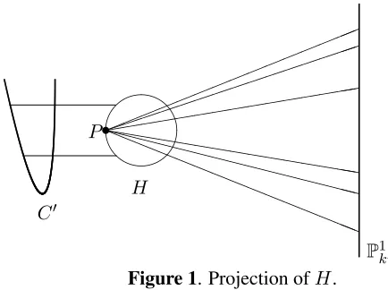
Figure 1. Projection ofH.
Our next problem is of a computational nature. The hyperelliptic curveC0 defined in (2.2) has two undesirable features: the first is that it is a singular curve and the second is that it is not of the formy2=h(x)forha separable polynomial in a single variablex. It is not practical to work on a curve of the formC0 is currently written in. Moreover, for our discrete logarithm transfer, we need to writeC0in the formy2 =h(x)so that we can apply our theorems recursively. So, we look at ways to re-write (2.2) into the formy2=h(x).
The standard way of doing this is to find a rational pointP and to compute a basis for the Riemann-Roch space
2P. This gives us a map, known as a pencil, fromC0 →P1kthat is also a double cover. It is a standard result from
here to derive an affine equationy2 =h(x)forC0 (see [1], I.6.A). However, we have a more efficient method; we will apply 19th century geometry that is rarely used to find algorithms.
We begin by looking at how Theorem 1 constructed the hyperelliptic curveC0. The reasonC0is hyperelliptic is that it covers the conicH :y2 =x2−w2. Now, if we look a bit closer atH, we see that it is a circle. We can find a
k0-rational point on this circle that is independent of the choice ofkork0: namely, the pointP = (x1, y1)given by
x1 = (−w2−1)/2andy1 = (w2−1)/2. If we use thisP as a base point on our circle, we can unwrap the circle into a line. Doing so (see e.g. page 7 of [32]), we obtain an isomorphismP1k0 → H given (locally) by sending a
fixed parametertforP1k0 to
(2.3) x= w
2+ 1
2 −
t(w2t+t+w2−1)
t2−1
(2.4) y= w
2−1
2 +t
w2+ 1− t(w
2t+t+w2−1)
t2−1
.
These formulas let us replaceH withP1k0 in the proof of Theorem 1. The curveC0 now covers thisP1k0 via this
isomorphism (see Figure 1). Returning to the proof of Lemma 1, we can compute the equation ofC0that coversH: this is just(Y −y1+y2)(Y +y1−y2)fory1 =
p
(x−w)f andy2 = p
(x+w)f. Further computation (again using thexandywe computed above) reveals that(Y −y1+y2)(Y +y1−y2) =Y2−2f(x−y). Now we have thatC0 coversHbyY2 = 2(x−y)f(x), but the right hand side is not yet a polynomial. To clear denominators, we replaceY byY(t−1)/(t2−1)dwhered=g(C0)/2 + 1. Collecting this into a single statement, we have the following.
Corollary 1. The curveC0 in Theorem 1 can be written as
(2.5) Y2 = 2(x−y)f(x)(t
2−1)g(C0)+2
(t−1)2 ,
wherexandyare given in (2.3) and (2.4) respectively. The right hand side is a polynomial ink0[t].
The equation forC0given in (2.5) is non-singular outside of points at infinity. This is in contrast to the equation forC0 given in Theorem 1. We will continue to letC0 denote the singular (projective) curve with affine equation given in Theorem 1.
k0 that has ak-isogeny Jac(C0) ∼ Jac(C)2. What we need to do next is to determine the relationship between the groupsΓ(Jac(C(k)))andΓ(Jac(C0(k0))). We will find out that there is a homomorphism between these two groups that has a small kernel. In the next section, we will show how to compute this homomorphism efficiently.
Since our varieties are defined over varying fields, we will consider all curves as defined over a fixed algebraic closure ofk0 (formally, we replaceC0 byC0⊗Speck0). We will letσdenote theqth power Frobenius whereqis the size ofk0. For any geometric pointQ= (x1, y1)on a hyperelliptic curve, letQ0 = (x1,−y1)(this notation is shorthand for the hyperelliptic involution). We will let(a, b1±b2)denote the divisor(a, b1+b2) + (a, b1−b2)on
C0. In the case thatb2is zero, we will simply add the same point twice. IfChas two geometric points at infinity, we will letD∞denote the sum of them; otherwise,C has one geometric pointP∞at infinity and we will letD∞
denote2P∞. It is clear that if we defineD0∞to be the same forσ(C), thenσ(D∞0 ) =D∞.
In the next result, we will look for a way to associate divisors ofCoverkwith divisors ofC0overk0. Intuitively, we want some form of a diagonal map on Jac(C)×Jac(σ(C))to stabilize the action ofσin the hopes of producing divisors onC0defined overk0. Recall that in the proof of Lemma 1, we had three curves:C1,C2,C3, and the glued curve. We also fixed mapsτi :Ci → P1k and, consequently, the mapτ : C0 → P1k. In this section, we have that
C =C1,σ(C) = C2, andH =C3. Also recall from Lemma 1 that we have two double coveringsπ1 :C0 → C andπ2 : C0 → σ(C). For the sake of notation, temporarily letπ denote either of these maps. It is well known thatπ∗π∗D = deg(π)D = 2Dfor a divisor D, wheredeg(π) = 2comes from our choice of π (see IV.ex.2.6 of[15]). The mapµ:Jac(C)×Jac(σ(C))→ Jac(C0)is given byπ∗1×π2∗once we have normalized our singular curves. Likewise, the map Jac(C0) → Jac(C)×Jac(σ(C))is given by (π1)∗ ×(π2)∗ once we have taken the normalizations. We can see from direct calculation (using classical derivatives) that the affine singular points ofC0
lie over the ramified points ofπ1:C→P1kwhich are sent to other ramified points ofCbyσ. By our construction, these points occur at exactly the roots of the polynomialf given in the definition ofC. At these points, the mapsπi will have different tangent directions for the same pointP and thus form a node onC0. The degree of the divisor summing up a blown up node onfC0 is2(this is made explicit in the proof of Corollary 1). Now we can prove our next result.
Theorem 2. There exist homomorphisms δ : Γ(Jac(C)(k)) → Γ(Jac(C0)(k0)) and δ0 : Γ(Jac(C0)(k0)) →
Γ(Jac(C)(k))such that the kernel of the composition δ0δ consists of all elements of order 2 on Γ(Jac(C)(k)).
Proof. LetP = (x0, y0)be an affinek-rational point onC. We will show how to mapP to a divisor onC0 over
k0. We start by defining the pointQ= (σ(x0), y1)onClying overσ(x0). The pointQneed not bek-rational, but it clearly must be defined in at most a quadratic extension ofk. IfP is ramified andx0is a root off, then define the divisorDto be the sum of the blown up points over the pointsP andσ(P)(which are defined on bothCand
σ(C)). This gives us a divisorDthat is fixed byσ. Otherwise, define the divisor
D= (x0, y0±σ(y1)) + (σ(x0), σ(y0)±y1))
on C0 (that the points described on Dare points of C0 follows trivially from the second definition of C0 in the proof of Lemma 1). If we look at this second definition ofD, it is immediate thatσ permutesx0 withσ(x0)and
y0 withσ(y0)(sincex0 andy0 are ink). As fory1, which may be in a quadratic extensionLofk, we know that
τ1(σ(σ(Q))) =σ(x0), soσ(σ(y1))is eithery1or−y1by Lemma 2. This shows us thatσpermutes the summands ofD, hence σ(D) = D. We now have that in both of our definitions ofD (one forP singular and one forP
non-singular) thatσ(D) =D. Moreover,σ generates both Gal(k/k0) and Gal(L/k0), soDis fixed by the entire Galois action in either case. This implies thatDis defined overk0 (see Lemma 4, Appendix 1, [27]). By Lemma 2, we could replace C byσ(C) andP by σ(P)and still obtain the same divisor D. Thus, we have a map from degree1divisors ofCto the divisors onC0 given byδ :P 7→(P, σ(P))7→D(whereDis defined above). Since we have thatdeg(D) = 4and we can translate Pic4(C0)to Pic0(C0)(over any base field), we can defineδas a map
Γ(Jac(C)(k))→Γ(Jac(C0)(k0)).
Now, if we push our divisorDback down toC (resp. σ(C)) in the case whereP is ramified, we get4P and otherwise, we get(π1)∗D = 2P +Q+Q0 (resp. (π2)∗D = 2σ(P) +σ(Q) +σ(Q)0). Subtracting2D∞(resp.
2σ(D∞)), we obtain2P−D∞(resp.2σ(P)−σ(D∞)). This tells us that ifα∈Γ(Jac(C)), then(π1)∗δ(α) = 2α.
Corollary 2. Using the notation above, #Jac(C)(k) =#Jac(C0)(k0).
Proof. In light of the previous result, we see that #Jac(C)(k)and #Jac(C0)(k0)are equal up to a factor of the form
2n. One can show that the points of order2on a hyperelliptic curvey2 =P(t)are completely determined by the factorization ofP(t)over the base field (see [2]). In our case, if we look at the equation forC0given in Corollary 1 and write it asC0 :y2 =P(t), we can see by elementary algebra that the linear factorx−rioff (from the curve
C :y2 = (x−w)f) corresponds to the (blown up) factor(t−1)2+ 2ri(t2−1) + (t+ 1)2w2ofP. Each factor ofPis of this form, except ifdeg(f)is even, whenP has a factor(t2−1)(corresponding to the blown up point at infinity). Now we have a simple relationship between the factors off and the factors ofP. Iff is of odd degreed
and hassfactors, thenP hasseven degree factors and degree2d≡2mod4. Otherwise,f is of even degree and
P hass+ 2factors, one of which has odd degree (e.g.(t−1)).
LetH : y2 = h(x) be a hyperelliptic curve over a finite field and suppose thath = Qs
i=1hi, where eachhi is irreducible (assume thath is separable). We define the 2-rank of Jac(H) to bedimZ/2Jac(H)[2](this is the dimension of theZ/2-vector space of all points of order2on Jac(H)over the finite field). In Theorem 1.4 of [5],
we have the statement that the2-rank of Jac(H)iss−2ifdeg(h)is even and somehihas odd degree; the2-rank iss−1 ifdeg(h) is odd or ifdeg(h) ≡ 2mod4and allhi have even degree; and the2-rank issotherwise. In our case, letf =Qs
i=1fifor irreduciblefi. Ifdeg(f)is odd, then(x−w)f is of even degree with an odd factor. In this case, Jac(C)has2-ranks−1. SinceP hasseven degree factors and degree2d≡ 2mod4, we have that Jac(C0)also has2-ranks−1. Ifdeg(f)is even, then(x−w)f has odd degree and2-ranks. In this case,P has even degree ands+ 2irreducible factors (one of which is linear), so Jac(C0)also has2-ranks.
Although it is tempting to conclude thatΓ(Jac(C0)(k0))andΓ(Jac(C)(k))are isomorphic, this is rarely the case. What we can show instead is that there is a special abelian variety defined overk0 that is isogenous to Jac(C0). Let
W be the Weil restriction of Jac(C)(overk) tok0. It is known thatW is an abelian variety of dimension2gthat is defined overk0(see Section 1 of [26]).
Corollary 3. There is a k0-isogeny W ∼ Jac(C0). IfL(t) is theL-polynomial of C overk, then L(t2) is the
L-polynomial ofC0overk0. Moreover, #C0(k0) =q+ 1.
Proof. It is known thatW can be defined as the abelian variety that represents the functor Resk/k0Jac(C)(S) =
Jac(C)(S×k0k)fromk0-schemesopto Sets. In particular, if we letS =Speck1for some finite extensionk1ofk0,
then we see that #W(k1) =#Jac(C0)(k1)(by using Corollary 2 over base extensions). This gives us ak0-isogeny
W ∼Jac(C0)(use Theorem 2.c, Appendix 1, [27]). Since theL-polynomial ofW isL(t2)ifLis theL-polynomial ofC (overk), we see thatL(t2) is theL-polynomial ofC0 overk0. Now, the number ofk0-rational points for a curve isq+ 1−P
αiwhere theαiare the roots of theL-polynomial of the curve overk0(see Appendix C, [15]). Since this sum is0onL(t2), we have that the number ofk0-rational points ofC0isq+ 1.
3. POINTCOUNTINGALGORITHMS
In this section, we construct three very simple algorithms for generating curves with a known number of rational points. In the case of genus2and4, we will even get the Zeta functions. Although interesting in their own right, the point counting algorithms will become essential to the discrete logarithm attack we will outline in the next section. For the definition of theL-polynomial and the Zeta function and their relationship, there are many references (see e.g. [25] or [15]), and we will not develop these ideas here (a worthy discussion would take an entire chapter). We will just mention that evaluating theL-polynomial at1gives us the order of the Jacobian. As before, we letFq be a finite field in odd characteristic and letFq2 =Fq[w]be a quadratic extension forw2 ∈Fq. LetCa curve defined by
(3.1) y2= (x−w)f
for any separablef ∈Fq[x]with roots outside±w.
Our first algorithm can be used to generate curves of any even genus with exactlyq+ 1points over a finite field.
Algorithm 1. Input:
(1) an odd prime powerq
Output:
(1) a hyperelliptic curve of genus2goverFqwithq+ 1points.
Procedure:
(1) randomly search for a non-squares∈Fq. Setw2=s.
(2) randomly search for a separable polynomialfof degree2g+ 1. (3) iff has eitherwor−was a root, return to the previous step. (4) Output equation (2.5) from Corollary 1 usingf andw.
Remark 1. The proof of correctness follows from Theorem 1, Corollary 1, and Corollary 3. The complexity of the algorithm amounts to a square root test, sampling separable polynomials of degree2g+ 1, and evaluating them at ±w. It is clear that the cost isO(glog(q))(see [31]). Ifggrows linearly andq grows exponentially, we can still generate these curves efficiently.
Our next algorithm can be viewed as a generalization and simplification of Algorithm 1 in [30]. We take in as input any hyperelliptic curve of the special form in Theorem 1. We are then able to construct a new hyperelliptic curve. In the case where we wish to generate genus2curves, we simply restrict to elliptic curves of the form given in Theorem 1.
Algorithm 2. Input:
(1) an odd prime powerq >3
(2) the valuew
(3) a curveCoverFq2 of the form (3.1) (4) theL-polynomialLofC.
Output:
(1) a hyperelliptic curve overFqwithL-polynomialL(t2).
Procedure:
(1) Output equation (2.5) from Corollary 1 usingf andw.
Remark 2. The proof is similar to the previous algorithm; using the results in Section 1, we simply apply Theorem 1 and Corollary 1 to constructC0, and then Theorem 2 and Corollary 3 to obtain the relation on theL-polynomial. In the special case whereCis an elliptic curve, we obtain a new algorithm for computing genus2curves. Beyond reducing the complexity of Algorithm 1 in [30] fromO(log2(q))operations overFqtoO(log(q)), our algorithm is able to sample odd and prime order Jacobians, whereas the previous algorithm (in [30]) could only generate even order Jacobians. One important application for these types of algorithms is finding genus2 curves suitable for public key cryptographic schemes (see [30] for a security analysis for curves of this type). For this purpose, it is important thatq be prime. Another application is to generate hyperelliptic curves for pairing based cryptographic schemes. In this case, C would have to be a (geometrically) supersingular hyperelliptic curve. (We will give examples in the Section 5.)
Now that we have seen how to make a genus2curve generator using the previous section, we outline how the previous section can generate similar algorithms for higher genus curves. The idea here is to start with an elliptic curveEover some fieldFq2k and construct a series of new curvesCi0overF
q2k−i, where each curveCi0satisfies the condition in Theorem 1. One can expect the equations to become more complicated asigrows, but for small genera one can produce extremely efficient curve generation algorithms using this idea. The genus4curve generator below demonstrates this. This algorithm is interesting by itself, and it has the extremely interesting feature that any of the curves it generates are cryptographically weak. Such a curve can be used to attack the elliptic curve used to construct it (see the next section).
To set things up, letFq2 ∼=Fq[w0], wherew0 is the square root of a non-square inFq, and supposew0−1is a non-square inFq[w0]. LetFq4 ∼=Fq2[w1]wherew12=w0−1. LetEbe the elliptic curve
(3.2) E:y2 = (x−w1)(x−r1)(x−r2),
Algorithm 3. Input:
(1) w0
(2) an integerh= #E Output:
(1) a hyperelliptic curve of genus4overFqwithL-polynomialq4t8+ (h−q4−1)t4+ 1or failure.
Procedure:
(1) IfEis not an elliptic curve, output failure.
(2) Otherwise, calculate the polynomialP ∈Fq[w0]as −1
8(((t−1)
2+ (t+ 1)2w2
0)(w20(t+ 1)2+ 3t2−2w−1)
(−2(t−1)2−(t−1)(t+ 3)w0−2(t+ 1)2w02+ (t+ 1)2w03)
(t(t+ 2)(w02−1) +w02+ 3))
(3) Output the hyperelliptic curveC :y2 =P.
Remark 3. This algorithm only fails whenr1,r2, and±ware not distinct. Like the previous algorithm, the formula can be computed inO(log(q))steps. The only thing that needs to be checked is that the intermediate curveC10 over
Fq2 is of the form required by Theorem 1. This amounts to checking long equations and using elementary algebra, so we omit the proof.
4. THE INDEX CALCULUS ATTACK
In Section 2, we mentioned a mapδthat could define a homomorphism from the Jacobian ofCto the Jacobian of
C0. Formally, the description ofδis given in Theorem 2. In this section, we will sketch an algorithm to compute it. For efficiency reasons, we will use Mumford’s representation of divisors (for background, see [4]). For simplicity, we will only describe the algorithm in the case that there is one rational pointP∞at infinity. For a rational point
P = (x0, y0)onC, recall thatP−P∞corresponds to the Mumford divisor[z−x0, y0]wherek(z)is the function field of the projective line covered by C. When we use polynomial interpolation in the following algorithm, we will always mean the polynomial of minimal degree passing through the specified number of points.
Algorithm 4. Input:
(1) a curveCoverFq2 of the form (3.1) (2) a divisorD= [z−x0, y0]onC (3) the curveC0from Algorithm 2.
Output:
(1) a divisorD0 in Mumford form onC0 such thatδ(D) =D0.
(1) Definea0(z) = (z−x0)(z−xq0)and definea(t) =a0(x)(t2−1)2wherexis as in Corollary 1. (2) ify0= 0, then return[1,0]. //this is a ramified point
(3) ifx0 ∈k0, then //this is a rational point that needs to be counted twice
(a) leta1(t)anda2(t)be the irreducible factors ofa(t)(they need not be distinct). (b) ifa1anda2are unique, replaceaiwitha2i.
(c) Letαibe the unique root ofai, setei= (α2i −1)(αi+ 1). (d) LetT be the tuple(e1Tr(y0), e2Tr(y0))
(e) LetGbe the polynomialy2=G(x)definingC0. (f) Setbi= (T[i]2+G)/(2T[i]).
(g) ifGmoda1 =b2i moda1then return[a1, bimoda1]. (h) ifGmoda2 =b2i moda2then return[a2, bimoda2].
(4) letRbe the list of roots ofa(t)over a splitting field (letRi denote theith coordinate). (5) letd0=
p
f(xq0)(xq0−w)over this extension (ignore the sign). (6) lete(t) = (t2−1)(t+ 1).
(a) if the test passes, append[(y0−d0)e(Ri),(y0+d0)e(Ri), Ri)]to matrixL. (8) if #Rows(L)<2orx0 ∈k0, then
(a) letbbe the polynomial interpolating the points(L1,3, L1,1),(Lp1,3, L p 1,2). (b) replacea(t)with its irreducible factor and return2[a(t), b]
(9) else letAinterpolate(L1,3, L1,1),(L2,3, L2,2),(Lp1,3, L p 1,1),(L
p 2,3, L
p 2,2). (10) and letBinterpolate(L1,3, L1,2),(L2,3, L2,1),(Lp1,3, L
p 1,2),(L
p 2,3, L
p 2,1). (11) ifGmoda(t) =A2moda(t), return[a(t), A].
(12) else return[a(t), B].
All of the computations preformed in the above procedure are just arithmetic manipulation of small degree poly-nomials and a few factorizations. The complexity of this algorithm is clearlyO(log(q))(see [31]). The proof of this algorithm is a consequence of the construction given in Theorem 2. To see this, note that at any step in the procedure, at least one root ofa(t)lies over the value ofx0in the covering mapfC0 →C. This means thata(t)is a polynomial that has roots over the locus of points overx0inP1k; there are at most4such points. What the algorithm is doing is testing all possible cases in this locus using the valuey0. Sinceδis a homomorphism, there is only one unique solution (otherwiseδ would map a point into a locus). The remaining details are minor. For example, if
x0 ∈k0, then we can improve the algorithm by splitting upa(t)and using the trace to avoid taking square roots. The final step is to outline a full attack. First, we sample at random an elliptic curve in the class given by (3.2). We repeat until we find a #Ewith a large prime factor, and if so, we take a random discrete logarithm instanceD,
D0 onE. We use Algorithm 3 for the choice ofw0used to sampleE to construct the hyperelliptic genus4curve
C0 overFq. Now we use the previous algorithm onDandD0twice to get to two divisorsD2, D02onC0 (here we may be forced to deal with points at infinity in a different way). A solution to the discrete logarithm problem on
D2andD02is only off by a factor of2when we apply it to the originalDandD0.
For the hyperelliptic curveC0 given in Algorithm 3, index calculus works by first finding rational points onC0
to form a strictly ordered setS ⊂C0(k0)of some large size. Once such a set has been fixed, one takes a discrete logarithm instance(D, D0)onC0and calculates, for each stepi, random numbers(αi, βi)of size less than the order of the Jacobian ofC0. One then computesDi=αiD+βiD0and converts this to Mumford notation[a(t), b(t)]. If the support ofDiis inS, then one collects(αi, βi)and the points in this support. This is the case ifa(t)splits and its rootsri form points(ri, b(ri))inS. For eachiwhere this occurs, we form a (usually sparse) matrixM such that each rowihas a number representing the multiplicity of these points (with respect to the given strict ordering onS). Once this linear system is large enough, we search through it to find a non-trivial vector in its kernel. Such a vector gives us the relationR=P
aiMi = 0, whereMi is theith row ofM. The expressionRcan be rewritten
asR = P
ai(αiD+βiD0) = 0, and from here we have PaiαiD = P−aiβiD0. If we letα = Paiαi and
β =P
aiβi, we have thatD=−β/αD0.
In our setting, we have a discrete logarithm problem(P, P0)onEthat is mapped to a discrete logarithm problem
(D2, D02)on a genus4curveC0. By adapting the index calculus method to mimic the number field sieve with the use of large primes, the amount of work required to solve a discrete logarithm problem on a genus4curve isO(q14/9)
(see [35]). In contrast, the amount of time running Pollard-Rho on the elliptic curve E we have constructed is
O(q2). We will leave it to future work to determine exactly how much of a security parameter increase is required in practice.
We can also offer a few improvements that may help in practice. Since we know #C0(k0) = q + 1, we can orderk0 ×k0 in some natural way, and we can let S be the factor basis of points up to some maximal number. This saves us from having to storeS. The second improvement is that we can computeαiPi+βPi0onEand map it to a divisor onC0. This saves us from having to use the slower algorithms in [4] for Jacobian arithmetic on a hyperelliptic curve. Another option is to instead computeS and map each divisor inS back toE and ignore C0
completely. We will leave further discussion to future work.
5. IMPLEMENTATIONS ANDEXAMPLES
then the distribution of their orders among the possible orders is still very mysterious (for conjectures and further discussion, see [13]). Depending on the application, control over the order is often desirable, and it is in these cases that one often assumes that the distribution has regularly occurring values of some desired type. For example, in elliptic curve public key cryptography, one often assumes that via a random search of elliptic curves, one will find prime order groups for a non-negligible portion of all elliptic curves (as the base field grows). In practice, this does seem to occur. The lack of proofs in this area requires us to give examples if we want to make claims about the types of curves we can generate. These examples give evidence that the desired orders can be found via a random search. In another type of distribution problem, it is very easy to single out supersingular elliptic curves from the class of all elliptic curves in characteristicp ≡3mod4. We will show how this can be used to construct supersingular hyperelliptic curves where there is a reduction of their discrete logarithm problems to the same problems in a finite field. At the end of this section, we will provide links to source code for all of our algorithms so that they can be tested against various distributions.
5.1. Weak Elliptic Curves and Points Counts. Algorithm 2 seems to be able to generate prime order Jacobians of genus2curves at a very fast rate. For one such example at 160 bits, we have the hyperelliptic curve
y2= 67353434412343231568661t6+ 266764643564099517354601t5+ 244021071497214277712230t4+ 311017899974232689949122t3+ 557134887168713724834785t2+ 537290912002427906501256t+ 246564062462488879689319
over the prime field GF(1207034207473389622886491). The Jacobian of this curve has the 160bit (probable) prime order
1456931578010913785349746263294406745202104698519.
We had to sample41elliptic curves of the form specified in Theorem 1 before it found a prime order elliptic curve; Algorithm 2 then gave us the equation seen above. In other situations, we have found them in as little as3random searches, and at other times it has taken around100.
From a cryptographic point of view, one can conclude that the hyperelliptic curve above has the same level of security as the prime order elliptic curve it was sampled from. To test the speed at which a standard public key exchange could be executed on these curves, we have implemented Cantor’s algorithms (see [4]) in a standard (and very basic) hyperelliptic curve package in C++ using the NTL/GMP libraries (see below for links to this source code). We have found that the speed to be competitive on limited hardware, but we will leave a full analysis for future work.
The next example shows two things. On the one hand, it shows us that we can also sample almost of prime order genus4 curves using Algorithm 3. On the other, it shows us that we can sample elliptic curves of almost prime oder that can be attacked with index calculus. For an example of Algorithm 3 in action, letw20 = 12499454285990
overGF(17592186044423)and consider the elliptic curve defined by
E :y2 =x3+ (17592186044422w1+ (12188339541165w0+ 12188339541164))x2+ ((5403846503258w0+
5403846503259)w1+ (16901862777098w0+ 4980906183389))x+ (690323267325w0+ 12611279861034)w1
overGF(175921860444234). This curve has the171bit prime factor
1995436902172302086412028343508819458313536173109093.
One can test thatEis ordinary and has no special features that would rule it out as undesirable from a cryptographic point of view. Algorithm 3 gives us the following genus4hyperelliptic curve.
C:y2 = 362258632462x10+8876727378392x9+1189989348357x8+1604531604165x7+8121691981760x6+
10448625566159x5 + 16506034668669x4 + 15707410711712x3 + 7302308550432x2 + 1913995000352x + 6027788515385
We will leave to future work exactly how much of a security parameter increase is required to protect these vulnerable elliptic curves. In practice, we can sample these weak curves quickly. Moreover, one can also readily produce examples of elliptic curves not in the class specified by Theorem 1 with the same number of points as one that is in this class. Since two elliptic curves with the same number of points are isogenous, we can attack curves not directly in the class of Theorem 1 once we have computed this isogeny. More computational experiments are necessary to determine if there is any hope of writing down exactly which types of elliptic curves must be avoided if they are to be used in public key cryptography.
5.2. Supersingular Hyperelliptic Curves. Another application of our algorithms is to use them to construct su-persingular curves (see [8] for background information). The existence of these curves is not resolved for all characteristics and for all genera (see [22]). Where they are known to exist, supersingular curves have an appli-cation to pairing based cryptography (see [3], [10]). From a discrete logarithm point of view, these curves should be considered very weak when compared to other elliptic curves; it is possible to reduce the discrete logarithm problem on these curves to a discrete logarithm problem in a finite field (see [24]). We will show how to use our algorithms to sample curves where the discrete logarithm is very weak in this sense, even though our curves will be of a higher genus. The fact that our approach generates hyperelliptic curves is interesting for two other reasons: the first is that supersingular hyperelliptic curves are interesting from the theory of moduli (see [22]), and the second is that they have an application to pairing and are more efficient to use than a general curve.
We will prove that every elliptic curve is of the form in Theorem 1 over at most a base extension. This should not be surprising from a geometric point of view: an elliptic curve is given by four distinct points and we can move any three of them by a fractional linear transformation ofP1. In what follows, we will require that the characteristic
of our base field is larger than3.
Lemma 3. Every elliptic curve can be written in the form given in Theorem 1 over at most a finite base extension.
Proof. Over a base extension,Ecan be written as
E :y2=t(t−1)(t−λ)
over somek. For allw∈k∗, we can show thatEis isomorphic over a finite extension ofkto a curve of the form
E0 :y2= (t2−ζ)(t−w)
forζ =λ2w2/(λ−2)2 ifλ6=−1andζ =w2/9otherwise. To see this, one just computes thej-invariants ofE
andE0and shows that they are the same. Thus, over a finite extension,EandE0are isomorphic.
To illustrate how this result can be used to manufacture supersingular hyperelliptic curves, recall that the curve
y2 = x3−xis supersingular overFp for allp≡ 3mod4(this is a simple calculation of the Hasse-invariant, see [33]). Using Lemma 3, this curve can be made into E : y2 = (t2 −w2/9)(t−w) forw the square root of a non-square inFp. We can now send this to Algorithm 2 to produce an explicit supersingular genus2curveC0over
Fp. A simple algorithm to go from Jac(C0)toE based on Theorem 2 would be the following.
Algorithm 5. Input:
(1) E:y2 =f
(2) C0
(3) A Mumford divisorD= [a(t), b(t)], wheredeg(a(t))≤2.
Output:
(1) a divisorD0 onEsuch thatδ0(D) =D0.
Procedure:
(1) Factora(x)into rootsα1,α2.
(2) Evaluateβi =x(αi)forxas in Corollary 1. (3) Collect the pointsPi= (βi,±
p
f(βi)), output thePithat createsDin Algorithm 4.
All divisors on a genus2curve can be represented by[a(t), b(t)]fordeg(a(t))≤2(see [4]). If we now apply the reduction in [24] toE, we have reduced the discrete logarithm problem on the divisors ofC0to that of a finite field.
REFERENCES
[1] E. Arbarello. M. Cornalba. P. Griffiths. J. Harris.Geometry of Algebraic Curves: Volume 1, Springer-Verlag, 1985. [2] E. Artin.Quadratische K¨orper im Gebiete der h¨oheren Kongruenzen, I, II. Math. Z. 19, (1924). Collected Papers, 1-94. [3] D. Boneh. M. Franklin.Identity-Based Encryption from the Weil Pairing, SIAM J. of Computing, 2003.
[4] D. Cantor.Computing in the Jacobian of a hyperelliptic curve, Mathematics of Computation 48, 1987.
[5] G. Cornelissen. Erratum toTwo-torsion in the Jacobian of hyperelliptic curves over finite fields, Arch. Math. 77, 2001. [6] M. Deuring.Die Typen der Multiplikatorenringe elliptischer Funktionenk¨orper, Abh. Math. Sem. Univ. Hamburg 14, 1941. [7] C. Diem.On the discrete logarithm problem in class groups of curves, Math. Comp., to appear.
[8] T. Ekedahl.On supersingular curves and abelian varieties, Math. Scand. 60, 1987.
[9] A. Enge.Computing Discrete Logarithms in High-Genus Hyperelliptic Jacobians in Provably Subexponential Time, Math. Comp., 2002.
[10] S. Galbraith.Supersingular curves in cryptography, Asiacrypt 2001, Springer LNCS 2248, 2001.
[11] S. Galbraith. M. Harrison. D. Morales.Efficient Hyperelliptic Arithmetic Using Balanced Representation for Divisors, ANTS, 2008. [12] S. Galbraith, F. Hess, N. P. Smart.Extending the GHS Weil descent attack, Eurocrypt 2002, Springer LNCS 2332, 2002.
[13] S. Galbraith. J. McKee.The probability that the number of points on an elliptic curve over a finite field is prime, Journal of the London Mathematical Society, 62, no. 3, 2000.
[14] P. Gaudry.An Algorithm for Solving the Discrete Log Problem on Hyperelliptic Curves, Eurocrypt 2000, Springer LNCS 1807, 2000. [15] R. Hartshorne.Algebraic Geometry, Springer-Verlag., New York, 1977.
[16] F. Hess.Computing Relations in Divisor Class Groups of Algebraic Curves Over Finite Fields, preprint, 2004.
[17] M. Jacobson. N. Koblitz. J. Silverman. A. Stein. E. Teske.Analysis of the Xedni calculus attack, Design, Codes and Cryptography 20, 2000.
[18] E. Kani. M. Rosen.Idempotent relations and factors of Jacobians, Math. Ann. 284, 1989.
[19] K. S. Kedlaya.Counting points on hyperelliptic curves using Monsky Washnitzer cohomology, J. Ramanujan Math. Soc, 2003. [20] N. Koblitz.Algebraic aspects of cryptography, Springer-Verlag, New York, 1998.
[21] N. Koblitz.Hyperelliptic Cryptosystems, Journal of Cryptology, Volume 1, Number 3, 1989.
[22] K. Li. F. Oort.Moduli of supersingular abelian varieties, Lecture notes in mathematics, Vol. 1680, Springer, 1998.
[23] Q. Liu.Algebraic Geometry and Arithmetic Curves, Oxford Grad. Texts Math., Oxford University Press Inc., New York, 2002. [24] A. Menezes. T. Okamoto. S. Vanstone.Reducing elliptic curve logarithms to logarithms in a finite field, STOC ’91, ACM, 1991. [25] J. S. Milne.Jacobian Varieties, InArithmetic Geometry(Storrs, Conn.), Springer-Verlag, 1984.
[26] J. S. Milne.On the Arithmetic of Abelian Varieties, Inventiones math. 17, 1972. [27] D. Mumford.Abelian Varities, 2nd ed, Oxford Univ. Press, Oxford, 1974.
[28] D. Mumford.The Red Book of Varieties and Schemes, Lect. Notes Math., Springer, New York, 1988. [29] J. Pila.Frobenius maps of Abelian varieties and finding roots of unity in finite fields, Math. Comput., 1990.
[30] T. Satoh.Generating Genus Two Hyperelliptic Curves over Large Characteristic Finite Fields, Eurocrypt 2009, Springer LNCS 5479, 2009.
[31] A. Sch¨onhage. V. Strassen.Schnelle Multiplikation großer Zahlen, Computing 7, 1971. [32] I. Shafarevich.Basic Algebraic Geometry 1, 2nd ed., Springer-Verlag, 1994.
[33] J. Silverman.The Arithmetic of Elliptic Curves, Springer-Verlag, 1985.
[34] J. Silverman.The Xedni Calculus And The Elliptic Curve Discrete Logarithm Problem, Designs, Codes and Cryptography 20, 1999. [35] N. Th´eriault.Index calculus attack for hyperelliptic curves of small genus, Asiacrypt 2003, Springer LNCS 2894, 2003.
[36] W. C. Waterhouse.Abelian varieties over finite fields, Ann. Sci. ´Ecole-Norm. Sup, 1969.