Mass Determination of
Elliptical Galaxies
Natalya Lyskova
Mass Determination of
Elliptical Galaxies
Natalya Lyskova
Dissertation
an der Fakult¨
at f¨
ur Physik
der Ludwig–Maximilians–Universit¨
at
M¨
unchen
vorgelegt von
Natalya Lyskova
aus Perm, Russland
Contents
Zusammenfassung xi
Summary xiii
1 Introduction 1
1.1 Mass determination techniques . . . 2
1.1.1 X-ray analysis . . . 2
1.1.2 Gravitational lensing . . . 3
1.1.3 Dynamical modeling . . . 4
1.2 The simple(st) mass estimators . . . 5
1.2.1 The virial theorem and virial-like estimators . . . 5
1.2.2 Estimators based on the spherical Jeans equation . . . 8
1.3 Structure of the thesis . . . 13
2 Simple recipe for estimating galaxy masses 17 2.1 Introduction . . . 18
2.2 Description of the method . . . 18
2.3 The sample of simulated galaxies . . . 20
2.3.1 Description of the sample . . . 20
2.3.2 Isothermality of potentials in massive galaxies . . . 21
2.3.3 Analysis procedure . . . 22
2.4 Analysis of the sample . . . 26
2.4.1 At a sweet point . . . 26
2.4.2 Simulated galaxies at high redshifts . . . 31
2.4.3 Mass from integrated properties . . . 31
2.4.4 Circular speed derived from the aperture velocity dispersion . . . . 33
2.4.5 Circular speed from X-ray data . . . 35
2.5 Testing the method on simulated galaxy clusters . . . 37
2.6 Discussion . . . 41
2.7 Conclusions . . . 44
3 X-ray bright elliptical galaxies 49
3.1 Introduction . . . 50
3.2 Description and justification of the method . . . 51
3.2.1 Rotation of galaxies. . . 53
3.2.2 An algorithm for estimatingVc . . . 56
3.3 Analysis . . . 56
3.3.1 M87, revisited. Illustration of the Method . . . 56
3.3.2 Observations and data reduction . . . 61
3.3.3 Circular speed from X-ray data. . . 62
3.3.4 Optical Rotation Curves . . . 68
3.3.5 Comments on individual galaxies. . . 70
3.3.6 Stellar populations: properties, M/L, contributions to the total mass 73 3.4 Discussion . . . 79
3.5 Conclusion . . . 83
3.6 Acknowledgments . . . 84
4 Performance of simple mass estimators for elliptical galaxies 89 4.1 Introduction . . . 90
4.2 Mass approximation formulae. . . 91
4.2.1 Local estimator. . . 92
4.2.2 Global estimator. . . 93
4.3 Tests . . . 94
4.3.1 Analytic models. . . 94
4.3.2 Tests on simulated galaxies. . . 101
4.4 Comparison of simple mass estimators with a state-of-the-art analysis. . . . 107
4.5 Mass proxy. . . 113
4.6 Discussions and Conclusions. . . 114
4.7 Acknowledgments . . . 115
5 Conclusions 119
List of Figures
1.1 X-ray and optical image of the Coma cluster . . . 3
1.2 Example of a strong gravitational lensing. . . 4
1.3 Aperture velocity dispersion as a function of aperture radius. . . 7
1.4 Projection of a spherical system along the line of sight . . . 9
1.5 σp(R) for I(R)∝e−7.67(R/R1/2)4 in Φ(r) =V2 c lnr+const . . . 10
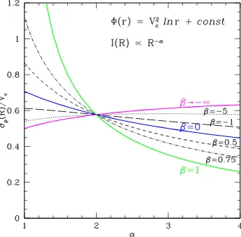
1.6 σp for I(R)∝R−α in Φ(r) = V2 c lnr+const as a function of α . . . 11
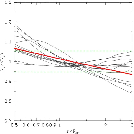
2.1 Circular velocity curves of massive simulated galaxies . . . 21
2.2 Excluding the satellites from the galaxy image . . . 22
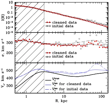
2.3 Influence of satellites onI(R),σp(R) and recovered Vciso . . . 23
2.4 Reff −M∗ relation as found for simulated galaxies . . . 25
2.5 Histograms of deviations ∆opt = Viso c −Vctrue /Vtrue c at different radii . . . 26
2.6 Examples of a relaxed galaxy and a galaxy with merger activity . . . 27
2.7 Histograms for the subsamples of simulated galaxies . . . 28
2.8 Histograms of deviations calculated for the subsample ‘MG’ at different radii 30 2.9 Accuracy of the derived potential of massive simulated galaxies . . . 32
2.10 σap(< R) within aperture of different radii as aVc-estimate . . . 34
2.11 Hot gas electron n(r),T(r), P =nkT and Vc(r) of a simulated galaxy . . . 36
2.12 Vc-eatimate from X-ray data for simulated galaxies . . . 37
2.13 Excluding the clumps from a hot gas density map of a simulated galaxy . . 38
2.14 Simple circular speed estimation in the simulated galaxy cluster . . . 39
2.15 The fraction of galaxy clusters as a function of the deviation . . . 40
2.16 Distribution of high-redshift galaxies from the subsample ‘MG’ . . . 43
3.1 Histograms of orientation-averaged deviations ∆opt for simulated galaxies . 54 3.2 Simple circular speed estimates of M87 . . . 58
3.3 SimpleVc-estimates for M87 Vs the state-of-the-art Vc-profiles . . . 59
3.4 The results of the SAO RAS 6-m telescope observations . . . 63
3.4 (continue) . . . 64
3.4 (continue) . . . 65
3.5 The effect of the abundance gradient on the X-ray derivedVc(r) . . . 67
3.7 The comparison of the Lick index profiles in NGC 4125 . . . 74
3.8 The comparison of the Lick index profiles in NGC 708 . . . 76
3.9 The radial variations of the stellar population metallicity . . . 77
3.10 The variations of the stellar population M/Lalong the radius . . . 78
3.11 The radial profiles of the surface mass density along the radius . . . 80
4.1 Typical profiles considered for a sample of analytical models . . . 96
4.2 Circular speed estimates for ‘ideal’ model galaxy . . . 97
4.3 Deviations of simple Vc-estimates from Vctrue for model spherical galaxies . 99 4.4 Dependence of deviations on properties of theVtrue c (r) and σp(R) . . . 100
4.5 Deviations for the localVc-estimator from the Vtrue c for simulated galaxies . 102 4.6 Deviations for the global Vc-estimator from the Vctrue for simulated galaxies 103 4.7 Observed correlations for simulated galaxies . . . 105
4.8 Deviation of the estimatedVc from theVtrue c as a function of Mvir . . . 106
4.9 α(R), σp(R) and VcSchw from the Schwarzschild modeling . . . 108
4.10 Comparison of simple Vc-estimates with VSchw c . . . 110
4.10 (continue) . . . 111
List of Tables
2.1 Summary of the methods discussed. . . 41
3.1 Sample of observed with the SAO RAS 6-m telescope elliptical galaxies . . 61
3.2 Log of the observations . . . 61
3.3 Vc-estimates for our sample of elliptical galaxies . . . 69
3.4 Metallicity gradient within and beyond the half effective radius. . . 75
3.5 Stellar masses and the fraction of dark matter (DM) within Rsweet . . . 79
3.6 Ellipticity and effective radius for the sample galaxies . . . 81
4.1 Main properties of Churazov et al. and Wolf et al. estimators. . . 95
4.2 Sample of real elliptical galaxies analyzed using the Schwarzschild modeling 107 4.3 SimpleVc-estimates and Vc from dynamical modeling . . . 112
Zusammenfassung
Die vorliegende Arbeit besch¨aftigt sich vorwiegend mit der Untersuchung und Weiteren-twicklung einer einfachen Sch¨atzfunktion f¨ur die Masse von fr¨uhen Galaxien, die sich f¨ur groe optische Galaxiendurchmusterungen mit mangelhaften und/oder ungenauen Daten eignen. Wir ziehen einfache und stabile Methoden in Betracht, die eine anisotropieun-abh¨angige Massenberechnung einer Galaxie aufgrund von Fl¨achenhelligkeit und projiziert-ern Geschwindigkeitsdispersionsdiagrammen erm¨oglichen. Es ist sinnvoll anzunehmen, dass eine grundlegende Degenaration der Anisotropie der Masse umgangen werden kann, ohne sich auf zus¨atzliche Beobachtungsdaten verlassen zu m¨ussen, allerdings nur in einem speziellen (charakteristischen) Radius, z.B. behandeln die Ans¨atze nicht die kreisf¨ormige Massendistribution. Zuversl¨assige Sch¨atzwerte in einem einzigen Radius k¨onnen wie folgt verwendet werden: (i) Kalibrierung anderer Methoden zur Massenberechnung; (ii) Sch¨atzung einer non-thermalen Zufuhr zum Gesamtdruck im Vergleich zu einem Sch¨atzwert der Masse einer R¨ontgengalaxie im gleichen Radius; (iii) Auswertung des Anteils der dunklen Materie im Vergleich zu der heller Materie; (iv) Ableitung der Steigung des Massenprofils, kom-biniert mit dem Sch¨atzwert der Masse eines starken Gravitationslinseneffekts; (v) Ersatz fr die Virialmasse.
Vor kurzem wurden zwei einfache Methoden ausgearbeitet: die lokale (Churazov et al. 2010) und die globale Methode (Wolf et al. 2010). Diese berechnen die Masse in einem spez-ifischen Radius und sind kaum von der Anisotropie stellarer Umlaufbahnen abh¨angig. Einer der Ans¨atze (Wolf et. al. 2010) verwendet die gesamte, nach der Leuchtkraft gewichtete Geschwindigkeitsdispersion und wertet die Masse in einem deprojizierten Halblichtradius aus, d.h. sie verl¨asst sich auf die globalen Eigenschaften einer Galaxie. Im Gegensatz dazu verwendet die Churazov et. al.-Methode lokale Eigenschaften, also logarithmische Kurven der Fl¨achenhelligkeit und der Geschwindigkeitsdispersionsdiagramme, und berechnet die Masse in einem Radius, in dem die Fl¨achenhelligkeit mit R−2
abnimmt (siehe Richstone und Tremaine 1984, Gerhard 1993).
2). Wenn man die globale Methode auf massive simulierte Galaxien mit einem ann¨ahernd flachen Geschwindigkeitsdispersionsdiagramm anwendet, kann man ebenfalls eine nahezu unverf¨alschte Sch¨atzung der Masse erzielen, obwohl die QMW-Abweichung geringf¨ugig gr¨oer ausf¨allt (≃ 14−20%), als fr die lokale Methode (Kapitel 4). Eine auff¨allige Abwe-ichung wird in der Ermittlung des charakteristischen Radius erwartet, da der Halblichtra-dius von dem RaHalblichtra-diusbereich fr die Analyse und der angewandten Methode abh¨angt.
Als n¨achstes habe ich die Sch¨atzfunktionen an einer Stichprobe einer echten fr¨uhen Galaxie, die schon eingehend mit dem neuesten dynamischen Modellverfahren analysiert wurde, analysiert. F¨ur diese Gruppe von Galaxien liegen die Sch¨atzwerte erstaunlich nah an den Ergebnissen der Schwarzschildmodelle, obwohl einige davon flach sind und langsam rotieren. Sobald die lokale Sch¨atzfunktion an das Beispiel angeglichen worden ist, betr¨agt die Abweichung von der im dynamischen Modellverfahren errechneten Ideal-masse ≈ 10% und die QMW-Abweichung ≈ 13% zwischen den verschiedenen Galaxien. Die Erwartungstreue kann mit Messunsicherheit verglichen werden. Desweiteren wird die Abweichung gr¨oßtenteils von einer einzigen Galaxie verursacht, die die h¨ochste Dichte in der Stichprobe aufweist. Schließt man diese aus der Stichprobe aus, vermindert sich die Verzerrung auf ≈ 6% und die QMW-Abweichung um ≈ 6%. Die globale Sch¨atzfunktion f¨ur dieselbe Stichprobe zeigt eine mittlere Abweichung von ≈ 4% mit einer geringf¨ugig gr¨oßeren QMW-Abweichung von ≈15% (Kapitel 4).
Angesichts der positiven Ergebnisse wende ich die lokale Sch¨atzmethode auf eine Stich-probe an, die f¨unf helle fr¨uhe R¨ontgengalaxien beinhaltet, die mit einem 6-m Teleskop in Russland beobachtet werden. Durch die Verwendung der ¨offentlich verf¨ugbaren Chandra-Daten ist es mir gelungen, das R¨ontgenmassenprofil mithilfe der Thesen der Sph¨arischen Symmetrie sowie des Hydrostatischen Gleichgewichts von heißem Gas abzuleiten. Ein Ver-gleich zwischen den Sch¨atzfunktionen der optischen- und R¨ontgenmasse erlaubte es uns, der non-thermalen Zufuhr zum Gesamtdruck, die beispielsweise durch microturbulente Gasbe-wegungen verursacht wurde, Grenzen zu setzen (der an die Stichprobe angeglichene Wert betr¨agt ≈ 4%). Sobald die aus der R¨ontgenstrahlung entstandene Kreisgeschwindigkeit f¨ur die non-thermale Zufuhr korrigiert wurde, lieferte die Diskrepanz zwischen der aus der R¨ontgenstrahlung entstandenen Kreisgeschwindigkeit VX
c und der optischen Kreis-geschwindigkeit f¨ur stellare Umlaufbahnen Viso
c Hinweise auf die orbitale Struktur der Galaxie. Zum Beispiel w¨urden kleine Radii VX
Summary
The work presented here focuses on the investigation and further development of simple mass estimators for early-type galaxies which are suitable for large optical galaxy surveys with poor and/or noisy data. We consider simple and robust methods that provide an anisotropy-independent estimate of the galaxy mass relying on the stellar surface brightness and projected velocity dispersion profiles. Under reasonable assumptions a fundamental mass-anisotropy degeneracy can be circumvented without invoking any additional obser-vational data, although at a special (characteristic) radius only, i.e these approaches do not recover the radial mass distribution. Reliable simple mass estimates at a single radius could be used (i) to cross-calibrate other mass determination methods; (ii) to estimate a non-thermal contribution to the total gas pressure when compared with the X-ray mass estimate at the same radius; (iii) to evaluate a dark matter fraction when compared with the luminous mass estimate; (iv) to derive the slope of the mass profile when combined with the mass estimate from strong lensing; (v) or as a virial mass proxy.
Two simple mass estimators have been suggested recently - the local (Churazov et al. 2010) and the global (Wolf et al. 2010) methods - which evaluate mass at a particular radius and are claimed to be weakly dependent on the anisotropy of stellar orbits. One approach (Wolf et al. 2010) uses the total luminosity-weighted velocity dispersion and evaluates the mass at a deprojected half-light radius, i.e. relies on the global properties of a galaxy. In contrast, the Churazov et al. technique uses local properties: logarithmic slopes of the surface brightness and velocity dispersion profiles, and recovers the mass at a radius where the surface brightness declines as R−2 (see also Richstone and Tremaine
1984, Gerhard 1993).
To test the robustness and accuracy of the methods I applied them to analytic models and to simulated galaxies from a sample of cosmological zoom-simulations which are similar in properties to nearby early-type galaxies. Both local and global simple mass estimates are found to be in good agreement with the true mass at the corresponding characteristic radius. Particularly, for slowly rotating simulated galaxies the local method gives an almost unbiased mass-estimate (when averaged over the sample) with a modest RMS-scatter of
analysis and applied methodology.
Next I tested the simple mass estimators on a sample of real early-type galaxies which had previously been analyzed in detail using state-of-the-art dynamical modeling. For this set of galaxies the simple mass estimates are in remarkable agreement with the results of the Schwarzschild modeling despite the fact that some of the considered galaxies are flattened and mildly rotating. When averaged over the sample the simple local method overestimates the best-fit mass from dynamical modeling by ≈10% with the RMS-scatter
≈ 13% between different galaxies. The bias is comparable to measurement uncertainties. Moreover, it is mainly driven by a single galaxy which has been found to be the most compact one in the sample. When this galaxy is excluded from the sample, the bias and the RMS-scatter are both reduced to ≈ 6%. The global estimator for the same sample gives the mean deviation ≈ 4% with the slightly larger RMS-scatter of ≈ 15% (Chapter 4).
Given the encouraging results of the tests I apply the local mass estimation method to a sample of five X-ray bright early-type galaxies observed with the 6-m telescope BTA in Russia. Using publicly available Chandra data I derived the X-ray mass profile assum-ing spherical symmetry and hydrostatic equilibrium of hot gas. A comparison between the X-ray and optical mass estimates allowed me to put constraints on the non-thermal contribution (sample averaged value is ≈ 4%) to the total gas pressure arising from, for instance, microturbulent gas motions. Once the X-ray derived circular speed is corrected for the non-thermal contribution, the mismatch between the X-ray circular speedVX
c and the optical circular velocity for isotropic stellar orbits Viso
c provides a clue to the orbital structure of the galaxy. E.g., at small radii VX
Chapter 1
Introduction
Since the beginning of the 20-th century mass measurements of galaxies and clusters of galaxies is a hot and actively discussed topic. Interest to ‘weighing’ galaxies and galaxies clustes has led to an extremely important discovery of dark matter. In 1933 Fritz Zwicky applied the virial theorem to the Coma galaxy cluster and found that the virial cluster mass is ≈ 400 times greater than the ‘visual’ mass estimated from the total brightness of the cluster. Zwicky calculations suggested that there must be some form of an unseen matter (‘dark matter’) which would be able to hold the cluster galaxies together. First observations of spiral galaxies rotation curves (Babcock, 1939; Mayall, 1951) showed no Keplerian velocity decrease in the outer regions in contradiction to expectations. This observation also had no significant influence on scientific community, rather details of the analysis (e.g., adopted distances) were questioned. Most astronomers in the ∼ 50−60s kept believing that disk galaxies had Keplerian velocities at moderate and large distances from the center. Thanks to progress in instrumentation, observations of hundreds extended rotation curves became available in ∼1980s, majority of which demostrated no Keplerian velocity fall. This fact played a major role in convincing the scientific community that there exist an unseen (dark) matter which accounts for a major part of the total mass of disk galaxies. It took ≃ 50 years to make the paradigm of the dark matter common and widely accepted. Dark matter emit/absorb electromagnetic radiation very weakly (if at all) and interacts with ordinary matter mainly gravitationally. Unfortunaly, up to now there is no reliable detection of dark matter particles in the Earth experiments, and galaxies and galaxy clusters retain the status of main laboratories for investigation of dark matter properties.
therein).
1.1
Mass determination techniques
A number of techniques have been developed in the past to investigate the mass distribu-tions in early-type galaxies. Each methods has its own set of assumpdistribu-tions and limitadistribu-tions. Comparison of mass profiles inferred from different techniques is necessary to get reliable estimates and to control systematic uncertainties, inherent in all methods. It also leads to interesting constraints on properties of elliptical galaxies, when possible biases are well un-derstood and systematic errors are under control. Let us briefly describe main approaches for analysis of early-type galaxies.
1.1.1
X-ray analysis
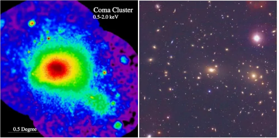
Massive elliptical galaxies (and galaxy clusters) are bright X-rays sources as found by the Einstein X-ray observatory (Figure 1.1 shows an example of a X-ray image of a galaxy clus-ter). X-ray observations of hot diffuse gas in these galaxies (as well as in galaxy clusters) allows one to probe the galaxy gravitational potential out to ∼ 10 kpc (∼ 10R1/2; R1/2
is the optical half-light radius) where observations in optical or radio bands are extremely challenging. Assuming hydrostatic equilibrium and spherical symmetry, with known (ob-tained from observations) gas number densityn(r) and temperatureT(r) profiles, one can estimate the galaxy mass:
1 ρ
dP dr =−
dΦ dr =
GM(< r)
r2 (1.1)
M(< r) =− kT r Gµmp
dlnn dlnr +
dlnT dlnr
, (1.2)
where ρ = µmpn is the gas density (mp stands for the proton mass, µ for the mean atomic weight), P = nkT is the thermal gas pressure (k is the Boltzmann constant) and Φ(r) is the gravitational galaxy potential.
1.1 Mass determination techniques 3
Figure 1.1: Hot X-ray emitting gas in the Coma cluster of galaxies as seen by ROSAT satellite is shown on the left (image credit: S.L. Snowden/ROSAT/MPE). The optical image of is on the right (image credit: O. Lopez-Cruz and I. Shelton/NOAO/AURA/NSF).
1.1.2
Gravitational lensing
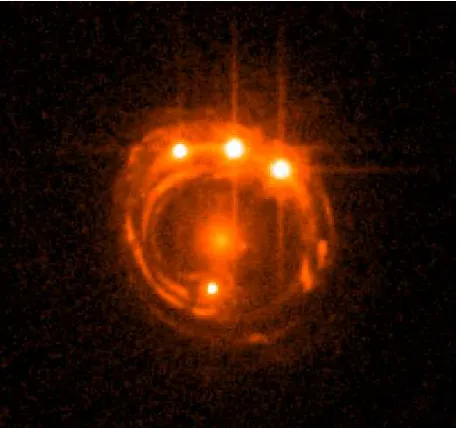
Gravitational lensing - bending the light rays by gravitational field - is the only method of mass determination, which can be applied to objects regardless of their composition and dynamical state (relaxed or disturbed). Depending on the deflection angle of light, gravitational lensing is divided into two regimes: strong and weak. If the source is a subject to strong lensing, the observer sees multiple images of the source and/or ring-like structures (Figure 1.2). Measuring the angular separation of images one can get an independent estimate of the total mass inside a cylinder with the Einstein radius RE =
s
4GM Dd(Ds−Dd)
c2Ds , where G is the gravitational constant, c - speed of light, M - the
lens mass, Dd and Ds are the distances from the observer to the lens and to the source respectively. Strong lensing offers an opportunity to infer the Hubble constant H by measuring the time delay between the source images and reconstructing a geometry of the gravitationally lensed system. An advantage of such method for the Hubble constant determination is that it probes directly the geometric scale of the system.
Figure 1.2: Example of a strong gravitational lensing. The quasar RXJ1131-123 as seen by the Hubble Space Telescope. Due to gravitational lensing the quasar appears as four point-like images connected by an Einstein ring. The lens galaxy is at the center of the ring.
developing.
1.1.3
Dynamical modeling
All methods that are based on modeling kinematic data of elliptical galaxies suffer from the fundamental degeneracy between the galaxy mass and the anisotropy of tracer orbits. The interpretaion of the observed velocity dispersion profile σp(R) alone is found to be ambigous due to the lack of single ideal tracers on known orbits.
Dynamical modeling using orbit superposition (Schwarzschild method, 1979) is consid-ered to be the state-of-the-art technique for the investigation of early-type galaxies which recovers the galaxy’s gravitational potential and orbital structure with an accuracy of .15% (e.g., Thomas et al., 2005).
1.2 The simple(st) mass estimators 5
parameters of the gravitational potential are varied, and the whole procedure is carried out again as long as the deviation of the resulting model from observational data reaches the minimum value.
The Schwarzschild technique allows one to obtain a radial distribution of a galaxy mass, to study the contribution of individual components (luminous matter, dark halo and supermassive black hole) to the galaxy gravitational potential. The method can be applied to any steady-state collisionless system. No assumptions on the orbit configuration is required. Derived distribution function in the six-dimensional phase space is guaranteed to be everywhere positive (= to be physically meaningful). The main challenge is to construct a representative library of orbits. The orbit-superposition technique is widely used for determining the mass distribution, dark matter fraction and orbit configuration of nearby early-type galaxies as well as for ‘weighing’ central black holes. The method is very sensitive to the quality and completeness of the observational data, and not all the model parameters are uniquely constrained. It is also computationally expensive. E.g. the Schwarzschild orbit-superposition analysis of the nearby massive elliptical galaxy M87 took over ∼37500 hours of cpu (Gebhardt and Thomas, 2009).
As the sophisticated detailed modeling requires high signal-to-noise observational data on the line-of-sight velocity moments it is applicable only to nearby galaxies. Large as-tronomical surveys of galaxies at different redshifts are extremely important for galaxy formation and mass assembly studies. For such surveys usage of detailed dynamical mod-eling is not practical/possible especially in a case of poor and/or noisy observational data. It is desirable to have simple and robust techniques based on the most basic observables that provide an unbiased mass estimate with a modest scatter.
Before moving to simple mass estimators let us note that recent studies based on dif-ferent approaches and their combitations suggest that the gravitational potential Φ(r) of massive elliptical galaxies is close to isothermal (e.g. Gerhard et al., 2001; Treu et al., 2006; Koopmans et al., 2006; Fukazawa et al., 2006; Churazov et al., 2010).
1.2
The simple(st) mass estimators
1.2.1
The virial theorem and virial-like estimators
Despite an enormous progress in a development of mass determination techniques, the scalar virial theorem is still widely used for analyzing spheroidal systems especially at high redshifts where detailed high-quality observational data are not availbale. The total mass of an isolated spherical system in a steady state can be expressed as (Binney and Tremaine, 2008)
M = 3
σ2
p
rg
G , (1.3)
σp2
=
R∞
0 σ 2
p(R)I(R)R dR
R∞
0 I(R)R dR
. (1.4)
Apart from its simplicity the main advantage of the scalar virial theorem is its inde-pendence from the anisotropy β of tracers’ orbits. Unfortunately, the value of rg depends on the total and luminous mass distribution of a system, making the formula (1.3) not practical for mass determintation of real systems. One way to overcome this problem is to express the gravitational radius in terms of observationally abailable half-light radius R1/2 under some assumptions on a stellar density. Spitzer (1969) noticed that a ratio
be-tween a 3D half light radius and the gravitational radius r1/2/rg ≈ 0.4±0.2 for different polytropes (for polytropic index between 3 and 5). This result has been confirmed by Mamon (2000); Lokas and Mamon (2001), who theoretically derived r1/2/rg ≈ 0.403 for
the Hernquist (1990) model. For a wide range of stellar light profiles (S´ersic, exponential, Plummer, King) the 3D half light radius r1/2 is related to the projected half light radius
R1/2 as r1/2 ≈1.3R1/2 (Ciotti, 1991; Spitzer, 1987). So the relation (1.3) can be rewritten
as
M ≈1.6
σ2
p
R1/2
G (1.5)
for common analytical stellar density profiles.
Another way to get rid of rg in the equation (1.3) is to assume the isothermal form of a gravitational potential Φ(r) = Vc2lnr+const. As mentioned above, approximate isothermality of elliptical galaxies is suggested by a number of recent indepent studies on kinematics, X-rays and gravitational lensing. Assuming Vc(r) = const the virial theorem further simplifies to
M(< r) = 3
σ2
p
r
G , (1.6)
giving the radial total mass profile which is based on a single observale quantity and rigorously independent of the anisotropy parameter β.
In any form the virial theorem approach requires determination of the luminosity-weighted square of the projected velocity dispersion over the entire galaxy or within large enough aperture. How large should be an aperture radius to ensure that σap2 (Rap) =
RRap
0 σ 2
p(R)I(R)R dR
RRap
0 I(R)R dR
is insensitive to the anisotropy, i.e. σ2ap ≈
σ2p
1.2 The simple(st) mass estimators 7
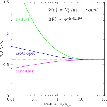
Figure 1.3: Aperture velocity dispersion σap as a function of aperture radius (normal-ized to the half-light radius) for a spherical galaxy described by the de Vaucouleurs law I(R)∝e−7.67(R/R1/2)
4
and an isothermal gravitational potential Φ(r) = V2
c lnr+const. The curves show the observed aperture velocity dispersion for different values of the anisotropy parameter: β = 0 (in blue), β → −∞ (in magenta) and β = 1 (in green). The minimum aperture radius required to ger a reliable estimate of
σ2
p
is ∼ 10R1/2. Adapted from
brightness distribution these three curves converge to the same value σap ≈ q σ2 p = Vc/√3 at very large aperture radius (∼10 half-light radii). For smaller aperture radii the σap is very sensitive to the anisotropy and can not be used as approximation for q
σ2
p
. Large apertures are available mostly for distant galaxies. For nearby ellipticals velocity dispersion profiles are typically observed out to ∼1−2 effective radii.
Having the surface brightness distributions and integral field kinematics of 25 nearby early-type galaxies Cappellari et al. (2006) calibrated the virial-like mass estimator in a form
M(< r1/2) =k
σ2
p
er1/2
G , (1.7)
where
σ2
p
e = σ
2
e is the luminosity-weighted line-of-sight velocity dispersion calcu-lated within a projected circular aperture of radius equal to an effective (half-light) radius R1/2. Comparing the simple virial-like mass estimators with masses from an axisymmetric
Schwarzschild models constructed for the same sample of galaxies, the coefficient k ≈2.5 has been derived, i.e. the mass within the 3D effective radiusr1/2 can be approximated as
M(< r1/2)≈1.9
σ2
er1/2
G ≈2.5 σ2
eR1/2
G , (1.8)
where r1/2 ≈ 1.33R1/2 used. Note this virial-like mass estimator implies the certain
methodology ofR1/2andσemeasurements (for details see Cappellari et al. 2006). The half-light radius and a total galaxy luminosity are obtained from a fit ofR1/4 (de Vaucouleurs)
growth curves to the aperture photometry and the σe is measured in a circular aperture of radius R1/2 centered on the galaxy.
1.2.2
Estimators based on the spherical Jeans equation
Another common approach to mass determination of elliptical galaxies is to use the station-ary non-streaming spherical Jeans equation which describes the motion of a collisionless system of test particles in a gravitational potential Φ(r). The Jeans equation relates to-gether the anisotropy parameter β, a volume density of tracers j(r) and a radial velocity dispersion σr(r) (Binney and Tremaine, 2008):
d dr jσ
2
r
+ 2β rjσ
2
r =−j dΦ
dr, (1.9)
where the anisotropy β(r) = 1 − σ2
t/σr2 (see Figure 1.4) for the spherically symmetric case (σt(r) is the tangential velocity dispersion). For a given β(r) one can derive M(< r) from the Jeans equation linking j(r) and σr(r) to the observable surface brightness I(R) and projected velocity dispersion σp(R) via the structural projection equation
I(R) = 2
Z ∞
R
j(r)r dr
√
1.2 The simple(st) mass estimators 9
Figure 1.4: Projection of a spherical system along the line of sight. r is the 3D radius, R stands for the projected radius,σt andσr are the radial and tangential velocity dispersions respectively.
and the anisotropic kinematic projection equation (Binney and Mamon, 1982)
σp2(R)I(R) = 2
Z ∞
R
1− R
2
r2 β
j(r)σ2
rr dr
√
r2−R2. (1.11)
For isotropic distribution of tracers’ orbits (β = 0) one can solve the spherical Jeans equation (1.9) and relate the mass M(< r) to the observables (I(R) and σp(R)) via the isotropic mass inversion equation (Mamon and Bou´e, 2010):
M(< r) =− r πGj(r)
Z ∞
r
d2(Iσ2
p) dR2
RdR
√
R2−r2, (1.12)
where a 3D stellar density is obtained from the Abel inversion equation:
j(r) = −1 π Z ∞ r dI dR dR √
R2−r2, (1.13)
In general, for any known anisotropy profile the equation of anisotropic kinematic pro-jection (1.11) can be inverted to yield the radial velocity dispersion profile σr(r), thus al-lowing one to derive the mass distribution of a spherical galaxy through the Jeans equation (1.9) in terms of double integrals of observable profilesI(R) andσp(R) (Mamon and Bou´e, 2010). Unfortunately, there is no direct and reliable way to deriveβ(r) from observational data without invoking an expensive detailed modelling.
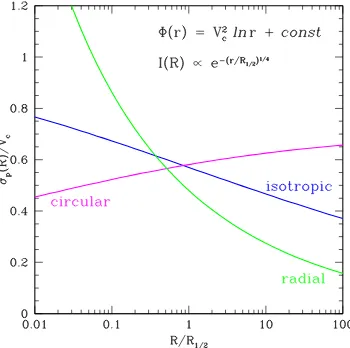
Richstone and Tremaine (1984) emphasized that the galaxy mass and the anisotropy still can be disentangled from the Jeans equation under some reasonable assumptions. For a spherical galaxy described by the de Vaucouleurs’s surface brightness distrubition I(R) ∝ e−7.67(R/R1/2)
4
1.2 The simple(st) mass estimators 11
isothermal gravitational potential Gerhard (1993) noticed that for the pure power-law surface brightness profile I(R) ∝R−α
) the projected velocity dispersion does not depend on the anisotropy for α = 2 (Figure 1.6). Combining these two notes, Churazov et al. (2010) proposed a simple mass estimator which determines the galaxy mass at the special radius which is close to R2 where I(R) declines as ∝ R
−2
. From the spherical Jeans equation (1.9) assuming Φ(r) = V2
c lnr+constone can derive an analytic relation between the circular speed (Vc2(r) = GM(< r)/r) and the local properties of I(R) and σp(R) for the cases of isotropic (β = 0), circular (β→ −∞) and radial (β = 1) orbits:
Vciso =σp(R)·p1 +α+γ Vccirc=σp(R)·
r
21 +α+γ
α (1.14)
Vcrad =σp(R)·
q
(α+γ)2+δ−1, where
α≡ −dlnI(R)
dlnR , γ ≡ − dlnσ2
p
dlnR, δ ≡
d2ln[I(R)σ2
p]
d(lnR)2 . (1.15)
A radius where Viso
c , Vccirc and Vcrad have similar values is the special radius where sensitivity of the method to the anisotropy β is expected to be minimal. Note, that for σp = const and not very steep surface brightness profiles (δ ≪α) the equations (1.14) can be simplified to:
Vciso=σp(R)·√α+ 1 Vccirc=σp(R)·
r
2α+ 1
α (1.16)
Vcrad =σp(R)·√α2−1.
So for nearly flat velocity dispersion profiles in the isothermal gravitational potential the galaxy circular speed (or mass) could be estimated at the radiusR2 whereI(R)∝R−2,
as pointed out by Gerhard (1993). For varying line-of-sight velocity disperion one can get an anisotropy independent estimate of the circular speed using the local properties of the observedI(R) andσp(R) profiles at the radius where analyticVc-profiles from the equations (1.14) have similar values.
1.3 Structure of the thesis 13
the mass within the radiusr3wherej(r)∝r−3 (which is close tor1/2 ≈1.33R1/2) is almost
independent of the assumed β(r) and can be approximated as
M(< r3)≈4
σ2
p
R1/2
G . (1.17)
In contrast to the Churazov et al. (‘local’) approach, this estimator requires averaging of the velocity dispersion out the the virial radius of the system and determination of the projected half-light radius, i.e. depends on the global galaxy properties. For the pure power-law surface brightness distribution and isothermal gravitational potential both methods gives the same circular speed estimate Vc =√3σp(R2) =
q
3
σ2
p
at the special radius R2 =r3.
1.3
Structure of the thesis
This thesis aims to investigate and further develop simple mass estimators for early-type galaxies which could be applied to analysis of large optical galaxy surveys.
Chapter 1 gives results of extensive tests of the local mass estimator on a sample of 65 cosmological zoom-simulations of individual galaxies. It is also demonstrated that the simple method could be succesfully applied to galaxy clusters where individual galaxies are used as mass tracers.
The application of the simple optical mass estimator to real X-ray bright elliptical galaxies is discussed in Chapter 2. Comparison of the simple estimate with the X-ray based and luminous mass profiles allows one to put constraints on the gas physics and configuration of stellar orbits. In this Chapter I estimate the magnitude of the non-thermal microturbulent motions of the hot gas, disentagle stellar and dark matter contributions to the total mass and characterize the distribution of stellar orbits for the analyzed sample of galaxies.
Chapter 3 presents a comparison of the simple local method with the global approach suggested by Wolf et al. (2010). To compare the methods I test them on a grid of analytical models, on samples of simulated galaxies and real early-type galaxies that had been already modelled using the Schwarzschild orbit superposition technique. A possibility to use the simple estimates as a proxy for a virial galaxy mass is also discussed.
Bibliography
Babcock H.W. 1939, Lick Obs. Bull., 19, 41 Binney J., Mamon G.A. 1982, MNRAS 200, 361
Binney J., Tremaine S. 2008, Galactic Dynamics, 2nd edn. (Princeton University Press) Buote D. A., Humphrey P. J. 2012, MNRAS, 421, 1399
Cappellar M., Bacon R., Bureau M., Damen M. C., Davies R. L., de Zeeuw P. T., Emsellem E., Falc´on-Barroso J., Krajnovi´c D., Kuntschner H., McDermid R. M., Peletier R. F., Sarzi M., van den Bosch R. C. E., van de Ven G. 2006, MNRAS, 366, 1126
Churazov E., Forman W., Vikhlinin A., Tremaine S., Gerhard O., Jones C. 2008, MNRAS, 388, 1062
Churazov E., Tremaine S., Forman W., Gerhard O., Das P., Vikhlinin A., Jones C., B¨ohringer H., Gebhardt K. 2010, MNRAS, 404, 1165
Ciotti L. 1991, A&A, 249, 99
Fukazawa Y., Botoya-Nonesa J. G., Pu J., Ohto A., Kawano N. 2006, AJ, 636, 698 Gebhardt K., Thomas J. 2009, ApJ, 700, 1690
Gerhard O.E. 1993, MNRAS, 265, 213
Gerhard O., Kronawitter A., Saglia R. P., Bender R. 2001, AJ, 121, 1936 Hernquist L. 1990, ApJ, 356, 359
Koopmans L. V. E., Treu T., Bolton A. S., Burles S., Moustakas L. A. 2006, ApJ, 649, 599 Lau E. T., Kravtsov A. V., Nagai D. 2009, ApJ, 705, 1129
Macci`o A.V., Dutton A.A., van den Bosch F.C. 2008, MNRAS, 391, 1940
Mamon G.A. 2000, in Combes F., Mamon G. A., Charmandaris V., eds, ASP Conf. Ser.Vol. 197, Dynamics of Galaxies: from the Early Universe to the Present. Astron. Soc. Pac., San Francisco, p. 377
Mamon G.A. and Bou´e G. 2010, MNRAS, 401, 2433
Mayall N.U. 1951, in The Structure of the Galaxy (Ann Arbor: Univ. Michigan Press), 19
Mo H.J., Mao S., White S. D. M. 1998, MNRAS, 295. 319 Nagai D., Vikhlinin A., Kravtsov A. V. 2007, ApJ, 655 98 Richstone D. O., Tremaine S. 1984, ApJ 286, 27
Schwarzschild M. 1979, ApJ, 232, 236 Spitzer L.J. 1969, ApJ, 158, L139
Spitzer L.J. 1987, Dynamical Evolution of Globular Clusters. Princeton Univ. Press, Princeton, NJ, p. 191
Thomas J., Saglia R.P., Bender R., Thomas D., Gebhardt K., Magorrian J., Corsini E.M., Wegner J. 2005, MNRAS, 360, 1355
Treu T., Koopmans L. V., Bolton A. S., Burles S., Moustakas L. A. 2006, ApJ, 640, 662 Wolf J., Martinez G.D., Bullock J.S., Kaplinghat M., Geha M., Mu˜noz R.R., Simon J.D.,
Avedo F.F. 2010, MNRAS, 406, 1220
Zhuravleva I., Churazov E., Kravtsov A., Lau E. T., Nagai D., Sunyaev R. 2013, MNRAS, 428, 3274
Chapter 2
Testing a simple recipe for estimating
galaxy masses from minimal
observational data.
Based on Mon.Not.R.Astron.Soc., 2012, 423, 1813
N.Lyskova, E.Churazov, I.Zhuravleva, T. Naab, L. Oser, O. Gerhard, X. Wu and on Astron. Nachr., 2013, 4-5, 360
N.Lyskova
Abstract.
The accuracy and robustness of a simple method to estimate the total mass profile of a galaxy is tested using a sample of 65 cosmological zoom-simulations of individual galaxies. The method only requires information on the optical surface brightness and the projected velocity dispersion profiles and therefore can be applied even in case of poor observational data. In the simulated sample massive galaxies (σ ≃200−400 km s−1
) at redshift z = 0 have almost isothermal rotation curves for broad range of radii (RMS≃5% for the circular speed deviations from a constant value over 0.5Reff < r < 3Reff). For such galaxies the
method recovers the unbiased value of the circular speed. The sample averaged deviation from the true circular speed is less than ∼1% with the scatter of ≃5−8% (RMS) up to R ≃ 5Reff. Circular speed estimates of massive non-rotating simulated galaxies at higher
redshifts (z = 1 and z = 2) are also almost unbiased and with the same scatter. For the least massive galaxies in the sample (σ < 150 km s−1) at z = 0 the RMS deviation is
≃ 7−9% and the mean deviation is biased low by about 1−2%. We also derive the circular velocity profile from the hydrostatic equilibrium (HE) equation for hot gas in the simulated galaxies. The accuracy of this estimate is about RMS ≃ 4−5% for massive objects (M > 6.5×10¹²M⊙) and the HE estimate is biased low by≃3−4%, which can be
2.1
Introduction
The accurate determination of galaxy masses is a crucial issue for galaxy formation and evolution models. Disentangling dark matter and baryonic matter of a galaxy permits test-ing the predictions of ΛCDM-cosmology and probtest-ing the mass function. An algorithm for deriving the mass of a spiral galaxy is straight forward - one just need to measure a rotation curve from gas or stars that can be safely assumed to be on circular orbits. For elliptical galaxies the situation is less simple. There is no ‘perfect’ (in terms of accuracy) tracer to measure the total gravitational potential. The main problem is the degeneracy between the anisotropy of stellar orbits and the mass. The shape of stellar orbits is not known a priory and different combinations of orbits may give the same distribution of light. Several different approaches for mass determination were proposed and succesfully implemented, like strong and weak lensing (e.g. Gavazzi et al., 2007; Mandelbaum et al., 2006), mod-elling of X-ray emission of hot gas in galaxies (e.g. Humphrey et al., 2006; Churazov et al., 2008), Schwarzschild modelling of stellar orbits, etc. Accurate data on the projected line-of-sight velocity distribution with information on higher-order moments enables an accurate determination of the mass distribution for nearby ellipticals (e.g. Gerhard et al., 1998; Thomas et al., 2011). However, in case of minimal available data detailed modelling is often not possible. Therefore it is important to find a method to measure galaxy masses with reasonable accuracy which gives an unbiased estimate when averaged over a large number of galaxies. In particular, it can be extremely useful while analysing large surveys, especially at high redshifts when detailed observational data of each individual galaxies are often not available.
The simplest way of estimating the mass of a galaxy is based on the projected velocity dispersion in a fixed aperture (e.g. Cappellari et al., 2006). A slightly more complicated approach is described in Churazov et al. (2010). To estimate the mass the only information required is the light profile and either the dispersion profile measurement or at least a reliable dispersion measurement at some radius. Testing this particular method on a sample of simulated galaxies is the subject of this paper. The main questions that we want to address are (i) What is the accuracy of this method? (ii) Does it give an unbiased result? (iii) What are the restrictions for application of this method?
The structure of the paper is as follows. In section 2.2, we provide a brief description of the method. In section 2.3 we describe the sample of simulated galaxies which is used to test the method. The analysis of the accuracy of the method is presented in section 2.4 where we also discuss alternative methods for determining the circular velocity. A summary on the bias and accuracy of the various methods is given in section 2.6 with conclusions in section 2.7.
2.2
Description of the method
2.2 Description of the method 19
The method is based on the stationary non-streaming spherical Jeans equation: d
drjσ
2
r+ 2 β
rjσ
2
r =−j dΦ
dr, (2.1)
wherej(r)1 is the stellar luminosity density,σr(r) is the radial component of the
veloc-ity dispersion tensor (weighted by luminosveloc-ity),β(r) = 1 − σ2
θ/σ2r is the stellar anisotropy parameter (σθ =σφ because of the assumed spherical symmetry) and Φ(r) is the gravita-tional potential of a galaxy.
While the stellar luminosity densityj(r) and radial dispersionσr(r) can not be observed directly they contribute to the two-dimensional surface brightness I(R) and the velocity dispersion σ(R) profiles:
I(R) = 2
Z ∞
R
j(r)r dr
√
r2−R2, (2.2)
σ2(R)·I(R) = 2
Z ∞
R
j(r)σ2
r(r)
1− R
2
r2 β(r)
r dr
√
r2−R2. (2.3)
Assumingβ(r) = const we note that β = 0 for systems where the distribution of stellar orbits is isotropic, β = 1 if all stellar orbits are radial and β → −∞ if the orbits are circular.
Assuming the logarithmic form of the gravitational potential Φ(r) = V2
c ln(r) + const and using local properties of givenI(R) andσ(R) one can calculate a circular velocityVc for three different types of stellar orbits: isotropic (σr =σφ=σθ, β= 0), radial (σφ =σθ = 0, β = 1) and circular (σr = 0, β → −∞). These relations are given by:
Vciso =σiso(R)·
p
1 +α+γ
Vccirc =σcirc(R)·
r
21 +α+γ
α (2.4)
Vcrad =σrad(R)·
q
(α+γ)2+δ−1, where
α≡ −dlnI(R)
dlnR , γ ≡ − dlnσ2
dlnR, δ ≡
d2ln[I(R)σ2]
d(lnR)2 . (2.5)
In case of noisy data on the dispersion velocity profile the subdominant terms γ and δ can be neglected, i.e. the dispersion profile is assumed to be flat, and equations (2.4) are simplified to:
Vciso =σiso(R)·
√
α+ 1
Vccirc=σcirc(R)·
r
2α+ 1
α (2.6)
Vcrad =σrad(R)·
√
α2−1.
Let us call a sweet spot the radius at which all three curves Viso
c (R), Vccirc(R) and Vrad
c (R) are very close to each other. One can hope that at the sweet spot the sensitivity of the method to the stellar anisotropy parameter β is minimal and the estimation of the circular speed at this particular point is reasonable. E.g. from equations (2.6) it is clear that in case of the power-law surface brightness profile with α = 2 and β = const the relation between the circular speed and the projected velocity dispersion does not depend on the anisotropy parameter (e.g. Gerhard, 1993). While the derivation of equations (2.4), (2.6) relies on the assumption about a flat circular velocity profile, tests on model galaxies with non-logarithmic potentials, non-power law behaviour of the surface brightness and line-of-sight velocity dispersion profiles and with the anisotropy parameter β varying with radius (Churazov et al., 2010) have shown that the circular speed can still be recovered to a reasonable accuracy. Now we extend these tests to a sample of simulated elliptical galaxies.
This method for evaluating the circular speed is not only simple and fast in implemen-tation but it also does not require any assumptions on the radial distribution of anisotropy β(r) and mass M(r).
The mathematical derivation of equations (2.4-2.6) can be found in Churazov et al. (2010). A similar approach and analytic formulae for kinematic deprojection and mass inversion also can also be found in Wolf et al. (2010) and Mamon et al. (2010).
2.3
The sample of simulated galaxies
2.3.1
Description of the sample
Simulations provide a useful opportunity to test different methods and procedures as all intrinsic properties of a system at hand are known. The main drawback of simulated objects is that they may not include all physical processes that take place in reality and thus may not reflect all complexity of nature. To test the procedure under consideration we have used a sample of 65 cosmological zoom simulations partly presented in Oser et al. (2010). These SPH simulations include feedback from supernovae type II, a uniform UV-background radiation field, star formation and radiative Hydrogen and Helium cooling but do not include ejective feedback in the form of supernovae driven winds. Present-day stellar masses of simulated galaxies range from 2.18×10¹⁰M⊙h−1to 28.68×10¹⁰M⊙h−1 inside 30 kpc. The
softening length used in simulations is about Rsof t=400 pc h−1, h = 0.72. Typically the
2.3 The sample of simulated galaxies 21
Figure 2.1: Circular velocity curves of massive galaxies (σ(Reff) > 200 km s
−1
) as a function of radius r. Individual rotation curves normalised to the speed averaged over [0.5Reff,3Reff] are shown in black, green dashed lines indicate the interval [1−RM S,1 +
RM S], where RM S = 4.9%, the red thick line represents the overall trend Vc ∝r−0.06 .
the observed scaling relations and their evolution with redshift. For detailed description of simulations and included physics see Oser et al. (2010).
To effectively increase the number of galaxies we have considered three independent projections of each galaxy. So the whole sample of simulated galaxies consists of 195 objects2.
2.3.2
Isothermality of potentials in massive galaxies
First of all we have found that massive galaxies in the sample have almost isothermal rotation curves over broad range of radii. To demostrate this statement (Figure 2.1) we have selected galaxies with a projected velocity dispersion at the effective radius σ(Reff)
(procedure of computation Reff is described in section 2.3.3) greater than 200 km s
−1 and
plotted their circular velocity curves Vc =pGM(< r)/r as a function of r/Reff. G is the
gravitational constant,M(< r) is the mass enclosed withinr andReff is the effective radius
of the galaxy. The circular velocity curves were normalised to the value of Vc averaged over r ∈ [0.5Reff,3Reff]. Three circular velocity curves that make the most significant
contribution to the RMS actually correspond to galaxies with the effective radius Reff <6
kpc. The fact that for these galaxies 0.5Reff is close to the softening length may affect the
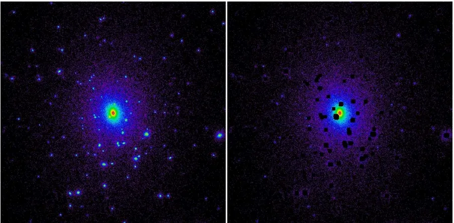
Figure 2.2: Excluding the satellites. 150 kpc×150 kpc. Left: Initial galaxy image. Right: Cleaned galaxy image.
scatter.
2.3.3
Analysis procedure
The analysis of each galaxy consists of several steps described below. Step 1: Excluding satellites from the galaxy image.
Usually an image of a simulated galaxy (the distribution of stars projected onto a plane) contains many satellite objects and needs to be cleaned. Exclusion of satellites makes the surface brightness and the line-of-sight velocity dispersion profiles smoother and reduces the Poisson noise associated with satellites. The algorithm we used for removing satellites is as follows: first, for each star a quantity w characterising the local density of stars (w∝ρ−∗1/3) and analogous to the HSML (the SPH smoothing length) was calculated and the array of these values was sorted. Then the (0.4·Nstars)thterm of the sortedw-array was chosen as a reference value wo. Nstars is a total number of stars in a galaxy and a factor in front of Nstars is some arbitrary parameter (the value 0.4 was chosen by a trial-and-error method). Stars with the 3D-radius r > 10 kpc and w < wo are considered as members of a satellite. After projecting stars onto the plane perpendicular to the line of sight we have excluded all satellites together with an adjacent area of 1.5 kpc in size. The inititial and final images of some arbitrarely chosen galaxy (the virial halo mass is ≃1.7×10¹³M⊙h−1)
are shown in Figure 2.2.
Step 2: Evaluating I(R) and σ(R).
2.3 The sample of simulated galaxies 23
the halo center. To calculate the surface brightness profile, corrected for the contamination from the satellites, we have first counted the number of stars in each annulus, excising the regions around satellites. The surface area of each annuli has been also calculated, excluding the same regions. The ratio of there quantities gives us the desired ‘cleaned’ surface brightness profile. The average line-of-sight velocity of stars and the projected velocity dispersion have been calculated similarly.
Importance of the ‘cleaning’ procedure and the resulting profiles of I(R) and σ(R) are shown in Figure 2.3. The surface brightness data (open circles correspond to the initial (‘uncleaned’) image and red solid circles to the ‘cleaned’ image) and the smoothed curves (the calculation of these curves is described in Step 3) are shown in the upper panel, the projected velocity dispersion profiles are shown in the middle panel. The true circular velocity Vtrue
c (r) (black solid curve) and recovered from the initial data (blue dashed line) and from ‘cleaned’ data (blue solid line) circular velocity for the isotropic distribution of stellar orbits Viso
c (the first equation in (2.4)) are shown in the bottom panel. The last curve is in better agreement with the true velocity profile. All results and figures in this paper are restricted to the region R >3.0 kpc.
Step 3: Taking derivatives.
To take derivatives we follow the procedure described in Churazov et al. (2010) in Appendix B. The main idea is that all data points participate in calculating the derivative but with different weights. The weight function is given by
W(R0, R) = exp
−(lnR0−lnR)
2
2∆2
, (2.7)
where R0 is the radius at which the derivative is being calculated and the parameter ∆ is
the width of the weight function.
Both observed and simulated surface brightness profiles are typically quite smooth so we have used ∆I = 0.3 to calculate the logarithmic derivative dlnI(R)/dlnR. For the line-of-sight velocity dispersion data we have used ∆σ = 0.5. With the assumed values of ∆ the local perturbations are smoothed out but the global trend of the profiles is not affected. Changing values ∆I and ∆σ in the range [0.3,0.5] does not significantly influence our final result3. The difference (in terms of circular velocity) is less than 1%. As an example the smooothed curves for the I(R) and σ(R) data in Figure 2.3 are calculated using this procedure.
We have also tested the influence of parameters of the presented smoothing algorithm. As long as the smoothed curve describes data reasonably well neither the functional form of the weight function nor other parameters (like higher order terms in expansion lnI(R) = a(lnR)2+blnR+cor σ(R) =a(lnR)2+blnR+c) significantly affect the final result.
Step 4: Estimating the circular velocity.
Applying equations (2.4) or (2.6) to the smoothed I(R) and σ(R) we have calculated Vc-profiles assuming isotropic, radial and circular orbits of stars. Then we have found a
2.3 The sample of simulated galaxies 25
Figure 2.4: Reff−M∗ relation. The blue solid line is the linear fit to data points from the
simulations. The green dashed line is the observed mass-size relation from (Auger et al., 2010).
radius (a sweet pointRsweet) at which the quantity (Vciso−V)2+ (Vcrad−V)2+ (Vccirc−V)2, whereV = (Viso
c +Vcrad+Vccirc)/3, is minimal. The value of the isotropic velocity profile at this particular point is the estimation of the circular velocity speed we are looking for. We take Viso
c as an estimate of the Vc(R) (rather than Vccirc or Vcrad) for two reasons. Firstly, at around one effective radius the dominant anisotropy for most elliptical galaxies isσzz < σRR ∼ σφφ (Cappellari et al. (2007)). The spherically averaged anisotropy is therefore only moderate (see also Gerhard et al. (2001), Figure 4). Massive elliptical galaxies are the most isotropic. Thus an isotropic orbit distribution is a much better approximation than purely radial or circular orbits. Secondly, the value of Viso
c is less prone to spurious wiggles in I(R) andσ(R).
The effective radius Reff is calculated as a radius of the circle which contains half of
the projected stellar mass, taking into account effects of cleaning. We found that in the simulated data-set the value of the effective radius depends on the maximal radius used to calculate the total number of stars in a galaxy. The problem is especially severe for the most massive galaxies as they have an almost power-law 3D stellar density distributionρ∗ ∝r−a with a≃3. In our analysis (in contrast to Oser et al. (2012)) we have not introduced any artificial cut-off and used all stars in the smooth stellar component (excluding substructure) of the main galaxies out to their virial radii for the calculation of the effective radius. The resulting effective radii as a function of total stellar mass (in logarithmic scale) are shown in Figure (2.4). The slope and the normalization of the Reff −M∗ relation are close to the
fit of SLACS data by Auger et al. (2010).
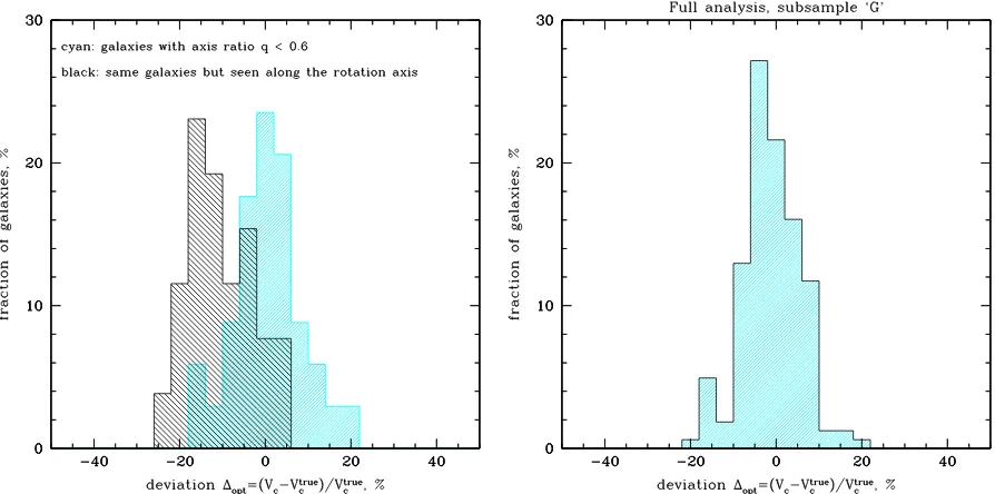
eigenval-Figure 2.5: The fraction of galaxies (in %) as a function of deviation ∆opt = Viso
c −Vctrue
/Vtrue
c evaluated via equations (2.4) at different radii: Rsweet (panel (A)),
Reff (panel (B)), 0.5Reff (panel (C)) and 2Reff (panel (D)).
ues of the diagonalised inertia tensor. The inertia tensor is computed within the effective radius without excluding substructures. We have found that q is not sensitive to our cleaning procedure as normally there are almost no satellites within Reff.
2.4
Analysis of the sample
2.4.1
At a sweet point
For each galaxy in the sample we have performed all steps described above and we have selected the radius at which the circular velocity curves for isotropic, circular and radial or-bits (equations (2.4)) intersect or lie close to each other. Then we have calculated the value of the isotropic speed Viso
c at this radius. To measure the accuracy of our estimates let us introduce a deviation from the true circular speed ∆opt= Viso
c −Vctrue
/Vtrue
c , where Vciso and Vtrue
2.4 Analysis of the sample 27
2.4 Analysis of the sample 29
to distinguish this method (based on optical data) from circular speed calculations based on X-ray data. We have plotted the number of galaxies (normalised to the total number of galaxies and expressed in %) versus the deviation ∆opt in a form of a histogram. To have an idea whether the method under consideration gives resonable accuracy, histograms for deviations at Reff, 0.5Reff and 2Reff are also shown. The whole sample (‘subsample A’) is
presented in Figure 3.6. The sample averaged value of the deviation ∆opt is slightly less than zero in all cases. For example, at the sweet point ∆opt = (−1.8±1.1)% while the RMS = 8.6%4.
Large deviations (∼30−40%) are seen only in galaxies with ongoing merger activity. The influence of mergers appears as ‘waves’ in the projected velocity dispersion profile. The example of such a system is shown in Figure 2.6 (right panel). The presence of such ‘waves’ indicates that the circular speed could be significantly overestimated (by a factor of ∼ 1.2−1.5), which is not surprising as the method is based on the spherical Jeans equations and the assumption about dynamical equilibrium is violated. When the profiles I(R) and σ(R) are smooth and monotonic the circular speed can be recovered with much higher accuracy (Figure 2.6, left panel).
The sample includes galaxies with different values of ellipticity. The axis ratio q (com-puted from the diagonalized inertia tensor within Reff) ranges from 0.19 to 0.99. To test
the possible influence of the ellipticity on the accuracy of estimates we have selected galax-ies with axis ratio q < 0.6. The resulting distribution as a function of the circular speed deviations is almost symmetric, unbiased, with RM S ≃ 8% (Figure 2.7). On the other hand, if we consider the same galaxies seen in a projection with the maximum value of the axis ratio q, we get the distribution appreciably biased toward negative values of the deviation (∆opt= (−10.2±1.6)%). The reason for this bias is rotation. When observing a galaxy along its rotation axis the projected velocity dispersion is appreciably smaller than for perpendicular directions. To further test this statement we have rotated each galaxy so that the principal axes of the galaxy (A≥B ≥C) coincide with the coordinate system (x,yand z, correspondingly) and analysed velocity maps for each projection. As a criteria for rotation we have used the anisotropy-parameter (v/σ)∗
= p v/σ
(1−q)/q, where v is the average rotation velocity of stars, σ is the mean velocity dispersion and q is the axis ratio (Binney, 1978; Bender and Nieto, 1990). If (v/σ)∗
>1.0 then the object is assumed to be rotating. We have found that the most massive simulated galaxies usually do not rotate or rotate slowly and show signs of triaxiality while less massive galaxies rotate faster and show signs of axisymmetry. This statement is in agreement with observational studies (e.g. Cappellari et al. (2007) and references therein). Moreover, the majority of rotating galax-ies appears to be oblate, rotating around the short axis. So for the oblate galaxgalax-ies observed along the rotation axis (and as a consequence seen in a projection with the axis ratio q close to unity) the method gives underestimated values of the circular speed. It should be noted that when observing the rotating galaxies along long axes the circular speed
esti-4x= P
x
N ,RM S=
r P
(x−x)2
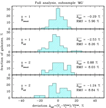
Figure 2.8: Left: Distribution of galaxies from the subsample ‘MG’ (massive galaxies with σ(Reff)>150 km s
−1
when merging and oblate galaxies observed along the rotation axis are excluded) according to their deviations. Deviations are calculated atRsweet (panel (A)),
Reff (panel (B)), 0.5Reff (panel (C)) and 2Reff (panel (D)). Right: The same histograms
but for the simplified version of the analysis (equations (2.6))
mate is slightly biased towards overestimation (Thomas et al. (2007) reached the similar conlusion). The average deviation for the subsample of oblate galaxies seen perpendicular to the rotation axis is biased high by ∆opt ≃(4.4±1.4)% with RMS = 6.3%.
To investigate possible projection effects on the results of our analysis we have picked one rotating galaxy (the virial halo mass is≃2.2×10¹²M
⊙h −1
) and calculated the surface brightness and the velocity dispersion profiles for different lines of sight. While the light profiles are quite similar, the velocity dispersion profiles may differ significanly when the line of sight is parallel to the rotation axis and perpendicular to it. We have calculated the average value of the circular speed estimates taking into account the probability of observing the galaxy at different angles. For the selected galaxy the average deviation from the true Vc is about −4.9% and the maximum deviation (when observing along the rotation axis) is about −25%.
It should be mentioned that the method under consideration was designed for recovering the circular speed in massive elliptical galaxies and it does not pretend to give accurate results for low-mass galaxies. In addition, not so many elliptical galaxies with σ <150− 200 km s−1 are observed (e.g. Bernardi et al., 2010).
It is convenient to distinguish low and high mass simulated galaxies by the value of the projected velocity dispersion at the effective radii. Let us call ‘massive’ galaxies with σ(Reff) >150 km s−1. If we apply our analysis to the subsample of massive galaxies and
2.4 Analysis of the sample 31
we get an unbiased distribution with RM S = 5.4%. The resulting histogram is shown in Figure 2.8, left image, panel (A). Estimations at other radii give slightly more biased and slightly less accurate results (Figure 2.8, left image, panels (B)-(D)).
Thereby we have marked out four subsamples - the whole sample without exceptions (‘A’ - all), the sample without merging or oblate galaxies seen along the rotation axis (‘G’ - good), the subsample of massive galaxies (‘M’ - massive) withσ(Reff)>150 km s
−1 and,
finally, the subsample of massive galaxies when merging and oblate galaxies observed along the rotation axis are excluded (‘MG’ - massive and good).
In case of missing or unreliable data on the line-of-sight velocity dispersion profile Churazov et al. (2010) suggest to apply a simplified version of the aforementioned analysis (equations (2.6)). By neglecting terms γ and δ we assume that the projected velocity dispersion profile is flat. Then the radius at which I(R) ∝ R−2 is the sweet point. The
resulting histograms for the subsample ‘MG’ are shown in Figure 2.8, right panel. It can be seen that data on the projected velocity dispersion plays noticable role in the analysis if the required accuracy is of order of several %. Neglecting its derivatives leads to a bias towards underestimated values ofVc (∆opt= (−4.0±1.1)% at the sweet point) and broader wings/tails (RMS = 6.4% at Rsweet) compared to Figure 2.8, left panel. Nonetheless, if
only the surface brightness profile and some data on the projected velocity dispersion are available the simplified version of the method seems to be a good choice.
2.4.2
Simulated galaxies at high redshifts
We have also tested the same procedure for galaxies at higher redshifts. Namely, at z = 1 andz = 2. The fraction of merging galaxies in the sample is larger at high redshift than at z = 0 and the number of stars in each halo is considerably smaller. Nevertheless, results are quite encouraging. For the subsample ‘MG’ the average deviation of the circular speed for the isotropic distribution of orbits at the sweet point (estimated via equations (2.4)) from the true one is close to zero and the scatter is modest. At redshiftz = 1 the average deviation is ∆opt = (−0.3±1.1)% and RMS = 6.0 %, at z = 2 ∆opt = (0.9±2.2)% and RMS = 8.0 %.
2.4.3
Mass from integrated properties
Asssuming the logarithmic form of the gravitational potential Φ(r) = V2
c lnr+const we can estimate the potential Φ over some range of radii up to a constant. To calculate the potential one needs to know the circular velocity profile. If we assume that this profile roughly coincides with the isotropic profile Viso
c over some range of radii (let us choose R∈[0.5Reff,3Reff] as a range of radii easily available for observations), we can define:
Φopt = R
Z
0.5Reff
Viso
c
2
Figure 2.9: Accuracy of the derived potential of massive galaxies (merging and oblate objects seen along the rotation axis are excluded). In cyan shown the histogram for the quantity ∆Φ = (1−κ)·100%, where κ= ∆Φtrue/∆Φopt. In black shown the histogram for
the deviation ˜∆opt of the estimated at the sweet point
Viso
c
2
from the true one [Vtrue
c ]
2