An argument for Hamiltonicity

An argument for Hamiltonicity

Vadym Fedyukovych

August 23, 2008

Abstract

A constant-round interactive argument is introduced to show exis-tence of a Hamiltonian cycle in a directed graph. Graph is represented with a characteristic polynomial, top coefficient of a verification polyno-mial is tested to fit the cycle, soundness follows from Schwartz-Zippel lemma.

1

Introduction

A protocol to show existence of a Hamiltonian cycle in a graph was intro-duced by Blum [Blu86, CF01]. Protocol uses binary challenges, and need to be repeated to achieve soundness. Protocols with ’large’ challenges achieve low soundness error without repeating; example is Schnorr pro-tocol with challenges chosen from a finite field.

We explore options resulting from algebraic structure of responses of a variant of Schnorr protocol. A protocol for Hamiltonian cycle is given in this report. Protocol is an argument on assumption of hardness of discrete logarithm problem. Protocol has a simulator algorithm, and is honest verifier perfect zero knowledge.

2

Preliminaries

Definition 1_{(Graph characteristic polynomial)}. _LetΓ be a labelled di-rected graph defined with a set of edgesE₍Γ)and a set of verticesV₍Γ). Non-zero labelswv ∈ F_{q,v ∈} V₍Γ)and flagsue ∈ {0, 1},e ∈ E₍Γ)are assigned to nodes and vertices. Consider a mapping to a ring of polyno-mials over finite field:

Γ→ f(x,y;Γ) =

∏

~eHT∈E(Γ)

(1+xwH+ywT) (1)

This definition appeared with a protocol for graph isomorphism. A similar characteristic polynomial was introduced with a protocol for vertex colorability. A related definition of set characteristic function appeared with set reconciliation [MTZ01].

Definition 2. _{Hamiltonian cycleis an alternating sequencev0,e1,v2,e2. . .vp} of vertices and edges of a graphΓ,|V₍Γ)|= psuch that all edges are dif-ferent, vp = v1, and vi =6 vj for all other pairs(i,j). We denote set of

edges that form the cycle withH₍Γ).

Lemma 1_{(Schwartz-Zippel [Sch80], a case of a univariate polynomial)}. Probability to choose a root of a nonzero polynomial f(z)of degree at mostdby samplingzat random from a domain of cardinalityD is at most _Dd.

3

Protocol

Consider a graph with a prime number of vertices: |V₍Γ)| = p. LetF_q be a field with a prime number of elements such that p|q−1. It follows a cyclic subgroup of order p exists in a multiplicative group of residue classesZq∗. Letap =1 (mod q),a6= 1.

To recognise a cycle, we assign labels to vertices such thatwj = aj, j= 0 . . .p, with indexjincrementing along the sequence. We also assign flags to edges such thatue = 1fore ∈ H₍Γ), andue = 0 for all other edges that are not part of the cycle.

Consider a polynomialfw(x,y,z)∈F_{q[X,Y,Z]for some{αv},αv ∈}F_{q,v ∈}V₍Γ): fw(x,y,z) =

∏

~eHT∈E(Γ)

(z+ (x(zwH+αH) +y(zwT+αT)))

Top coefficient of fw(x,y,z)is graph characteristic polynomial:

fw(x,y,z) =

n

∑

k=0

fk(x,y)zk, n= |E₍Γ)|, fn(x,y) = f(x,y;Γ)

Consider another polynomial fu(x,y,z)∈F_{q[X,Y,Z]for someβe∈}F_q, fu(x,y,z) =

∏

~eHT∈E(Γ)

(z+ (zue+βe)(xwH+ywT))

Top coefficient of fu(x,y,z)is characteristic polynomial of the cycle in the graph:

fu(x,y,z) =

n

∑

i=0

Let{Θ_v},{Φ_e}be responses of Okamoto protocol [Oka92] for commit-ments to labels and flags:

Θ_v=swv+αv

Φ_e=tue+βe Consider averification polynomial:

F(x,y,s,t) =

_∏

~eHT∈E(Γ)

(ts+Φ_e(xΘ_H+yΘ_T)) (2)

Anyone can produce an estimate ofF(x,y,s,t)using Verifier’ challenges and Prover’ responses. Verifier tests that top coefficient ofF(x,y,s,t)is

Ca(x,y) =

p−1

∏

j=0

(1+xaj+yaj+1) (3)

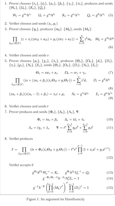
Common input is graphΓ, groupG_{, and group membersg,h. Auxiliary} input of Prover is a sequence of graph vertices that is a cycle. Protocol is shown of Figure 1.

Lemma 2_{(Recognising Hamiltonicity)}. _{A Hamiltonian cycle exists in} a graphΓ_,|V₍Γ)|= pfor some primep,p|q−1if, and only if labels wv,v ∈ Γcan be assigned with{aj}for somea ∈ Zq∗,ap = 1, a 6= 1 such that

∃(Γ′ ⊂Γ): f(x,y;Γ′)≡ p−1

∏

j=0

(1+xaj+yaj+1) (4)

Proof. It is clear that labels wv = aj can be assigned to vertices along the sequence indexed withjfor any givenasuch that characteristic poly-nomial of the cycle will be of the form (4), in case a cycle exists. We show that any subgraph with characteristic polynomial (4) is a Hamiltonian cy-cle.

We observe that characteristic polynomial is a product ofplinear poly-nomials that are relatively prime to one another. It follows there are ex-actlypedges in such a graph, such that each edge connects a vertex la-belled withajand a vertex labelled withap+1. It follows that vertices and edges form a sequence.

We also observe there are exactly p different values of the form aj, j= 0 . . .p−1, such that the sequence never crosses itself.

Fromap_{= a}0_{it follows that the last vertex in the sequence is the same}

as the first one, such that sequence is a cycle.

Lemma 3 _(Soundness). _{Probability for an honest Verifier to accept} for any Prover and any graphΓwithout Hamiltonian cycle running protocol shown on Figure 1 is at most 4|E(Γ)|+_q2|V(Γ)| over random choices of Verifier.

Proof. We show that Prover responses are estimates of polynomials that are linear in challenge, flags used are chosen from{0, 1}with probability at least1−2

q, and that fa(x,y)6≡0for

fa(x,y) =Ca(x,y)− f(x,y;Γ′)

with probability at most 2n+_q2p.

Consider a Prover capable of producing responsesΘ′, Ω′ to a chal-lengessuch that

gΘ′hΩ′W−s= R, Θ′ 6=Θ_, Ω′ 6=Ω

for

Θ=sw+α, Ω=sr+γ

W = gwhr, R= gαhγ

and for somew,r,α,γ ∈ F_{q. It follows such a Prover is also capable of} taking a logarithm using his responses as follows:

log_h(g) =−Ω ′_−Ω

Θ′_−Θ

We consider it infeasible for a polynomial Prover to produce valid re-sponsesΘ_,Ωother than estimates of polynomials that are linear both in challenge of Verifier and in value committed.

Consider a Prover capable of producing responsesΦ_,∆to a challenge tsuch that

g−Φ(Φ−t)h−∆NtE=1

for

Φ=tu+β

∆=tδ+π

N =gτhχ, E=gρhλ

for some u 6∈ {0, 1} and for some δ,β,π,τ,ρ,χ,λ ∈ F_{q. It follows} ft(z)6≡0for anyβ,τ,ρ:

From Schwartz-Zippel lemma it follows there is at most 2_q probability to choose a root of ft(z)at random: ft(t) = 0. It also follows that such a Prover is capable of taking a logarithm in case ft(t) 6= 0 using his responses as follows:

log_h(g) = ∆−χt−λ

ft(t)

We consider it infeasible for a polynomial Prover to produce valid re-sponsesΦ,∆ such that ft(t) 6= 0. It follows there is at most 2_q proba-bility for an honest Verifier to accept at (14) for any Prover and for any flag u6∈ {0, 1}over random choices of challenget.

Consider a Prover capable of producing responses{Φ_e},{Θ_v},Ψ to challengesxc,yc,s,tsuch that

g−Fh−Ψ n−1

∏

k=0

(Mk)sk

!tn

n−1

∏

i=0

(Di)ti =1

for

F=

∏

~eHT∈E(Γ)

(ts+Φ_e(xcΘ_H+ycΘ_T))−tnsn p−1

∏

j=0

(1+xcaj+ycaj+1) Φ_e=tue+βe

Θ_v=swv+αv

and for some Ψ. From Lemma 2 it follows fa(x,y) 6≡ 0 for any sub-graph ofΓ. From Schwartz-Zippel lemma it follows there is at most 2_qp probability to choose a root of fa(x,y)at random: fa(xc,yc) =0. In case

fa(xc,yc)6= 0it follows fs(z)6≡0for any{sk}:

fs(z) = fa(xc,yc)sn+

n−1

∑

k=0

skmk

From Schwartz-Zippel lemma it follows there is at most n_q probability to choose a root of fs(z)at random: fs(s) =0. In case fs(s)6=0it follows

fst(z)6≡0for any{di}:

fst(z) = fs(s)zn+

n−1

∑

i=0

zidi

is capable of taking a logarithm in case fst(t)6=0using his responses as follows:

log_h(g) = (fst(t))−1(Ψ−tn n−1

∑

k=0

skηk− n−1

∑

i=0

tiµi)

We consider it infeasible for a polynomial Prover to produce valid re-sponses{Φ_e},{Θ_v},Ψ such that fst(t) 6= 0. It follows there is at most

2n+2p

q probability for an honest Verifier to accept at (15) for any Prover and for any graph without Hamiltonian cycle over random choices of chal-lengesxc,yc,s,t.

We consider a Prover passing verification equations such thatft(t) =0 for any edge due to unlucky choice of challenge t, or fst(t) =0 (due to choice of challenges xc,yc,s,t) to win the game. This probability esti-mate is sufficient for our purposes; a better estiesti-mate may be developed by considering options and strategies available to Prover.

We conclude there is at most2_qpprobability for such a Verifier to accept while choosing(xc,yc), n_q while choosings, and 2_qn+ n_q while choosing t, unless Prover is capable of taking logarithms in the group used. This probability is exponentially small in group order bitsize.

Lemma 4_{(Of knowledge)}. _{Protocol shown on Figure 1 has an} extrac-tor algorithm, and is of knowledge.

Extractor is based on rewinding procedure: make Prover respond to two different challenges without choosing another set of initial random coins. All labels and flags are produced with an algorithm developed for Schnorr protocol [Sch89].

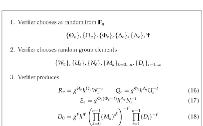
Lemma 5_{(Zero knowledge)}. _{Protocol shown on Figure 1 has a} simu-lator algorithm, and is honest verifier zero knowledge.

Simulator algorithm is shown on Figure 2. Probability distribution for group elements{Rv},{Qe},{Ee},D0is flat due to{Ωv},{∆e},{Λe},Ψ chosen independently with flat distribution.

4

Discussion

References

[Blu86] Manuel Blum. How to prove a theorem so no one else can claim it. In International Congress of Mathematicians, pages 444–451, 1986.

[CF01] Ran Canetti and Marc Fischlin. Universally composable com-mitments. InCRYPTO, pages 19–40, 2001.

[Luc94] Stefan Lucks. How to exploit the intractability of exact tsp for cryptography. InFSE, pages 298–304, 1994.

[Luc95] Stefan Lucks. How traveling salespersons prove their identity. InIMA Conf., pages 142–149, 1995.

[MTZ01] Y. Minsky, A. Trachtenberg, and R. Zippel. Set reconciliation with nearly optimal communication complexity. In Interna-tional Symposium on Information Theory, page 232, 2001. http://citeseer.ist.psu.edu/minsky00set.html.

[Oka92] Tatsuaki Okamoto. Provably secure and practical identifi-cation schemes and corresponding signature schemes. In CRYPTO, pages 31–53, 1992.

[Sch80] J. T. Schwartz. Fast probabilistic algorithms for verification of polynomial identities. J. ACM, 27(4):701–717, 1980.

1. Prover chooses

{

rv

}

,

{

δe

}

,

{

αv

}

,

{

βe

}

,

{

γv

}

,

{

πe

}

, produces and sends

{

Wv

}

,

{

Ue

}

,

{

Rv

}

,

{

Qe

}

:

Wv

=

gwvhrv Ue

=

guehδe Rv

=

gαvhγv Qe

=

gβehπe (5)

2. Verifier chooses and sends

(

xc,yc

)

3. Prover chooses

{

η_k

}

, produces

{

m_k

} {

M_k

}

, sends

{

M_k

}

:

∏

~eHT∈E(Γ)

(

z

+

xc

(

zwH

+

αH

) +

yc

(

zwT

+

αT

)) =

n

∑

k=0

zkm_k M_k

=

gmk_hηk

(6)

4. Verifier chooses and sendss

5. Prover chooses

{

µi

}

,

{

χe

}

,

{

λe

}

, produces

{

Θv

}

,

{

Ωv

}

,

{

di

}

,

{

Di

}

,

{

τe

}

,

{

ρe

}

,

{

Ne

}

,

{

Ee

}

, sends

{

Θv

}

,

{

Ωv

}

,

{

Di

}

,

{

Ne

}

,

{

Ee

}

:

Θ_v

₌

swv

+

αv Ωv

=

srv

+

γv (7)

∏

~eHT∈E(Γ)

(

zs

+ (

zue

+

βe

)(

xcΘH

+

ycΘT

)) =

n

∑

i=0

zidi Di

=

gdihµi

(8)

(

zue

+

βe

)(

z

(

ue

−

1

) +

βe

) =

τez

+

ρe Ne

=

gτehχe Ee

=

gρehλe (9)

6. Verifier chooses and sendst

7. Prover produces and sends

{

Φ_e

_}

,

{

∆_e

_}

,

{

Λ_e

_}

,Ψ:

Φ_e

₌

tue

+

βe ∆e

=

tδe

+

πe (10)

Λ_e

₌

tχe

+

λe Ψ

=

tn

n−1

∑

k=0

ηksk

+

n−1

∑

i=0

µiti (11)

8. Verifier produces

F

=

_∏

~eHT∈E(Γ)

(

ts

+

Φ_e

(

xcΘH

+

ycΘT

))

−

tnsn p−1

∏

j=0

(

1

+

xcaj

+

ycaj+1

)

(12)

Verifier accepts if

gΘv_hΩv_W−s

v

=

Rv gΦeh∆eUe−t

=

Qe (13)

g−Φe(Φe−t)_h−Λe_Nt

eEe

=

1 (14)

g−Fh−Ψ

n−1

∏

k=0

(

M_k

)

sk !tn

n−1

∏

i=0

1. Verifier chooses at random fromF_q

{

Θ_v

_}

_,

_{

Ω_v

_}

_,

_{

Φ_e

_}

_,

_{

∆_e

_}

_,

_{

Λ_e

_}

_,Ψ

2. Verifier chooses random group elements

{

Wv

}

,

{

Ue

}

,

{

Ne

}

,

{

Mk

}

k=0...n,

{

Di

}

i=1...n

3. Verifier produces

Rv

=

gΘvhΩvWv−s Qe

=

gΦeh∆eUe−t (16)

Ee

=

gΦe(Φe−t)hΛeNe−t (17)

D₀

=

gFhΨ

n−1

∏

k=0

(

M_k

)

sk !−tn

n−1

∏

i=1

(

D_i

)

−ti (18)