Video Face Recognition via Learned Representation on Feature-Rich key Frames

Video Face Recognition via Learned Representation on

Feature-Rich key Frames

Ambavaram Narayanamma & Chandra Mohan Reddy Sivappagari

(M.Tech Scholar)1 _{, (Associate Professor)}2

Department of Electronics and Communication Engineering1,2

JNTUA College Of Engineering Pulivendula, Pulivendula, Andhra Pradesh-516390,India2

[email protected]_{, [email protected]}2

A

BSTRACT

Nowadays, facial verification based authentication has become an important area of research in law enforcement and surveillance applications to combat widespread occurrences of security threat incidents,. It is satisfactory that the existing methodologies have marked great verification results at equal error rate, but have poor results at lower fault acceptable rates Therefore further research is required to increase verification performance while lowering the fault acceptance rate.

This paper, introduces a new face matching algorithm, that constitutes 1) Discrete Wavelet Transform and Entropy calculations for getting feature-rich key frames of a video .Then,

2)A Deep Learning Architecture, that consists of a Stacked Denoising Sparse Autoencoder (SDAE) and deep Boltzmann machine (DBM); is helpful for feature extraction..finally After completion of all these steps 3) a multilayer Feed Forward Neural Network System has been used as a classifier to get proper verification result.

The output is analyzed on two different openly accessible databases, YouTube Video Faces and Android Mobile Phone Database a type of point and shoot challenge(PaSC).

Results shows that the algorithm is successful: 1) in achieving sharpen increase in performance compared to histogram based frames, arbitrary frames, or frame collection with no reference image eminence measures 2) joint feature learning in SDAE and sparse and low rank regularization in DBM contributes to improve the face verification rate. The suggested method yields the success rate of matching faces about 95% s at equal error rate for

the You Tube Video Faces database, and it is possible to achieve even better results for PaSC database on the other hand.

Index Terms—Entropy, Autoencoder, Joint learning, Restricted Boltzmann Machine, Neural network

I.

I

NTRODUCTION

FACE identification of video has become highly petinent in authentication measures. Like many international games implements face detection based security system to check and identify individuals uniquely by using face verification methods of videos .

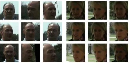
Fig. 1. The snaps are images from the PaSC video showcase the of quality of data present in a video, a subset of frames.

of a video clips where the facial areas have been found and trimmed. A single frame of a video can just have limited data, while collective frames bag a handful amount of data about the face relating to its look under the impact of regular covariates, for example, enlightenment, posture, and demeanors. Therefore a tough and thorough video face verifier is prerequisite.

Video face recognition has been broadly weighed and a few algorithms have been put forth.

The video face recognition is mainly categorised into two types

(1) set-based video face recognition

(2) Sequence based video face recognition

The set-based methodologies consider a video as an arrangement of pictures (outlines) which are then demonstrated and coordinated utilizing an assortment of approaches. These methodologies may not use the worldly data enclosed by a video, i.e. the request of casings in the first video may not make any difference. Then again, grouping based methodologies are particularly intended to use transient data of the video. These methodologies show the video as a grouping of pictures and impose arrangement characterization systems for recognition.

For correlation, the outcomes are for the most part given an account of benchmark databases, for example, YouTube face database (YTF), and as of late created Point and Shoot Challenge (PaSC) database . the existing calculations have achieved superior on YouTube video confront database]. In any case, the convention of this database by and large

requires existing detailing the outcomes at meet equal error rate(EER) . From an execution viewpoint, the calculations are needed to limit fault allowable rate(FAR) or fault reject rate (FRR).

.

Fig.2. shows the performance variations of the previous and proposed methods at EER and at 1%FAR on the YouTube faces database.

The outcomes of some previous works on You Tube faces databases are depicted in Fig. 2 . It is apparent that there is an immense gap in the execution at low false acknowledges rates when contrasted with execution at EER. But for many security associated applications like video surviallance, it is strongly wanted to attain very high performance of verification with lower false allowable rates Therefore, we can declare that an additional research is required to enhance the verification rate particularly at lower false allowable rates.

Fig.3. Block diagram of the stages drawn in the projected facial verification method .

Contributions

Of The

Research

As a rule, video face recognition includes coordinating every one of the casings introduce in two recordings. however, not all edges are similarly instructive and a few casings may experience the ill effects of low picture quality or outrageous varieties because of gesture, expressions, and focusses As it were, it is exceedingly likely that highlights obtained from such frames may result in fault outcomes..

Along these lines, it is fundamental to pick and operate the high data oriented frames of a video correctly and viably . To address some of these confinements and to enhance the general execution flow, we develope a new video confront acknowledgment calculation that uses a packaging assurance process, trailed by a profound learning design for highlight extraction and coordinating as showed in Fig. 3. The principal commitment of this examination is a novel calculation for obtaining wealthy feature-highlight based casings, that evaluates include lavishness in light of entropy [4] in the wavelet space and empowers better choice of

edges for acknowledgment when contrasted with conventional no-reference biometric entity means .

2. The next commitment is planning a fresh joint element learning structure which can be used to consolidate highlights processed in a profound system. In the suggested deep architecture, we consolidate the mid portrayals registered by an auto encoder as input to a joint portrayal layer. This joint portrayal is used to hold the educational highlights of various granularities and is utilized as contribution to a Deep Boltzmann Machine (DBM) that translates and upgrades the consolidated data to make a profound feature vector for every input face..

The learnt joint portrayal is contribution to a neural system for arrangement. The viability of the proposed calculation is assessed on two huge freely accessible benchmark databases: the YouTube Faces (YTF) video and Andriod mobile phone (PaSC) video .

[1] UIDAI Aadhar-authentication: Facial acknowledgment innovation (FRI) has ascended as an attractive reply for address various existing provisions for recognizing and the check of character claims. It joins the assurance of other biometric structures, which try to append character to solely unmistakable features of the body, and the more conspicuous value of visual surveillance systems. This report develops a socio-political examination that frameworks the specific and social-coherent abstract takes a shot at FRI and addresses the fascinating troubles and stresses that go to its change, evaluation, and specific operational uses, settings, and goals.

.

[2] Stan Z. Li, Anil K. Jain: Recognizing faces in free recordings is an errand of mounting significance. While clearly identified with confront acknowledgment in still pictures, it has its own particular interesting attributes and algorithmic prerequisites. Throughout the years a few strategies have been proposed for this issue, and a couple of benchmark informational collections have been amassed to encourage its examination. In any case, there is a considerable hole between the real application needs and the present best in class. In this paper we make the supplementary commitments.

(a) We present a colossal database of checked melodies of faces in exams assessment, uncontrolled circumstances (I. Digital on the. 'Inside the wild'), the 'YouTube Faces' database, together at the side of benchmark, combine coordinating tests1.

(b) We make utilization of our benchmark to evaluation appear at the execution of any huge variety of present video go up against affirmation frameworks. Presently,

(c) We show represent depict a one of a kind set-to-set appraisal measure, the Matched History Similarity (MBGS). This lien is appeared to surprisingly embellish execution at the benchmark tests.

III.

SUGGGESTED

FACE

RECOGNITION METHOD

The proposed work mainly consistsof three stages: One is frame selection, Second feature extraction through deep learning , and finally third is face verification using a classifier. Fig.3 gives the overview of our proposed work..

A. Entropy Driven Frame Selection

To extort discriminative features from a video, frame based processing is chosen, however, all frames are not appropriate for face verifcation while a few frames are hazy due to noise, blur, and occlusions, and may not contribute to consistent facial information and may affect the recognition performance. Ideally such frames should not be considered for feature extraction and matching [5]. Also, a simple video 8KB of duration of 5s results in large numberof of frames nearly 100-250. And subsequent frames hold high redundant information and processing all frames of a video increase computational density. To overcome this entropy based frame selection is preffered to establish a subclass of frames which is more suitable for face verification..

The video segmented into frame clusters and By using Principle Component Analysis (PCA), it selects the most representative frame from every cluster. Stop et al. [2] proposed by using active appearance models. Here with the estimation of pose and minimal motion blur it selects the frame. To create super resolved frames, utilizes optical flow.

part. Therefore we need only the facial region, remaining parts of the image does

Fig.4. distribution of Feature-highness value of various frames in a video.

not interrupt with the projected method. With standard deviation and mean image is normalized.

Fig.4. illustrates Feature-highness distributions of a video. Probably the most feature rich frames(values near 1) and least feature rich frames (values near 0) are introduced for examine. We can observe that the frames with high fidelity scores a higher feature richness value and the poor casings which exhibit curios, for example, impediment and obscure are assigned a low score of feature highness..

Given equation shows the computation of preprocessed image I:

[𝐼𝐴𝑃1, 𝐼𝐻𝑂1 𝐼𝑉𝑟1, 𝐼𝐷𝑔1] = 𝐷𝑊𝑇(𝐼) (1)

Here, 𝐼𝐴𝑝 denotes the approximation or estimation

coefficients and 𝐼𝐻𝑂 denotes the detail coefficients in

horizontal sub band, 𝐼𝑉𝑟denotes the detail coefficient

in vertical sub band and 𝐼𝐷𝑔denotes the detail

coefficient in diagonal sub band.

Another level DWT is applied on the first level , IAp1, coefficients as takes after:

[𝐼𝐴𝑃2, 𝐼𝐻𝑂2 𝐼𝑉2𝑟, 𝐼𝐷𝑔2] = 𝐷𝑊𝑇(𝐼𝐴𝑃); (2)

Here, I Ap2 and [IHo2 , IV r2 , IDg2 ] denotes the next level DWT estimation and detail coefficients of information picture IAP individually. DWT is helpful to empower multi-determinational investigation of the given picture. The main stage DWT represents the coefficients for the better points of interest of the picture, and the nextlevel DWT figures out the universal highlights .

For an images of size 80 × 100 and below, there is no need for third level DWT as it is unfit to hold proper edge-details. That’s why we prefer only two level DWT in this proposed method. For the region of image, entropy gives the pixel intensity value variation. To assess the feature richness of frames, entropy is calculated with the help of both 2 levels of DWT coefficients. For this initially a DWT band is devided into 3*3smaller windows and then entropy H(k) is computed for window k as.

𝐻(𝑘) = − ∑ 𝑃(𝐾𝑖)

𝑛

𝑖=1

log2 𝑃(𝐾𝑖) (3)

here, n denotes the whole count of pixel esteems, and p(κi) denotes the likelihood mass capacity for κi which indicates the likelihood occurances of pixel esteem κi in the nearby area. For window κi of size Mκ × Nκ. P(ki) is

𝑃(𝐾𝑖) = 𝑛(𝐾𝑖) 𝑀𝑘× 𝑁𝑘

(4)

Here, nκi indicates the quantity of pixels present in window having value κi. The entropy estimation of every window is added to obtain the component feature-wealth estimation of a band.

𝐻(𝐹) = ∑(|𝐻(𝑖)|

𝜔

𝑖=1

) (5)

band and Hi represents the I th window entropy. The final score of image I, H F(I), is acquired by combining the individual band feature richness estimations.

𝐻𝐹(𝐼) = 𝐻 𝐹 ( 𝐼′𝐴𝑃 ) + 𝐻 𝐹( 𝐼′𝐻𝑂 ) + 𝐻 𝐹 (𝐼′𝑉𝑟 )

+ 𝐻 𝐹 ( 𝐼′𝐷𝑔 ) + 𝐻 𝐹 (𝐼𝐻𝑂)

+ 𝐻 𝐹( 𝐼𝑉𝑟 ) + 𝐻 𝐹( 𝐼𝐷𝑔 ) (6)

Given a video V, the component extravagance score of an edge fi is spoken to as H F( fi). Since the score of each casing relies upon the circulation of force esteems in a casing, it is vital to standardize the chance to denotes to the’element abundance esteem’ to the I th outline fi, it is calculated with MIN-MAX standardization.

𝑚𝑖 =𝐻 𝐹( 𝑓 𝑖 ) − MIN(𝐻𝐹) MAX(𝐻𝐹) − MIN(𝐻𝐹) (7)

Where, HF signifies all the component extravagance scores for the video V and MIN (HF) and MAX(HF) signify the base and greatest esteems in HF, individually. More estimations of ‘mi’ imply a more component rich edge. Fig. 4 demonstrates the element abundance circulation a recording of a video having different pose,focuss,expressions from the YouTube Faces database, alongside test edges of high, normal, and low element wealth esteems. Once the score of each casing is registered, versatile edge determination is performed to decide the ideal arrangement of edges to signify a video. Let σ m indicate the standard deviation and μm signify the mean relating to the arrangement of highlight lavishness estimations for video V. The best outlines are chosen for check, ϕi is figured for each edge

𝜑𝑖 = {1 𝑖𝑓 𝑚𝑖 ≥ 𝜇𝑚 + 𝜎𝑚

2 0 𝑜𝑡ℎ𝑒𝑟𝑤𝑖𝑠𝑒

} (8)

Φi is a binary set developed for each frame that assigns value 1 or 0 accordimg to its feature abundance value mi is greater or lesser than the bound mentioned in the equation (8).

each casing with ϕ = 1 is chosen for a video. And are only considered for further process of joint

learning architechure explained in the following segment.

B. Joint Learning Architecure for Feature

Extraction

After the component rich edges are acquired, the following stage includes highlight extraction and coordinating. This paper, suggests a Stacked Denoising sparse Auto Encoders (SDAE) and Deep Boltzmann Machine (DBM) driven calculation that can submit great outcomes with constrained preparing information while at the same time having the capacity to use extra preparing information to additionally enhance execution.

1) Stacked Denoising Sparse Autoencoder and Deep Boltzmann Machines:

An auto encoder is anural network used for dimensionality reduction; that is for feature selection and extraction The encoder is deterministic mapping g𝜃 that transforms input vector x𝜖 𝑅𝛼 into feature f (latent representation). This computation given below.

𝑓 = 𝑔 𝜃 (𝑋) = 𝑠 (𝑊. 𝑋 + ∆) (9)

where 𝜃 𝑖𝑠 encoder parameter set, s denotes the sigmoid, w denotes the d × d weight matrix, and ∆ 𝑖s the balanced vector of order d. Using a decoder g𝜃,’, feature f is transformed back to input vector 𝑋̂ of order d.

𝑋̂ = 𝑔′𝜃′ (𝑓) _{= 𝑠 (𝑊}′_{. 𝑓 + ∆}′_{) (10)}

where, 𝜃′ indicating the decoder parameter set so that 𝑎𝑟𝑔𝑚𝑖𝑛_{‖𝑋 − 𝑋̂‖}

2 2

(11)

‖𝑋 − 𝑋̂‖₂2+ 𝛽 ∑ 𝐾𝐿(𝜌 ∥ 𝜌𝑗̂ )

𝑗

(12)

ρ denotes sparsity parameter, ρ ˆ j is the common activation of the j th hidden unit, K L(ρ ˆ ρ j ) = ρ log ρ ρ ˆ j + (1 − ρ) log 1 1− ˆ −ρ ρj is the K L- difference, and β is the sparsity punishment term. K L uniqueness calculates the contrast between a genuine likelihood dispersion and its estimate the Littler estimations of ρ and bigger estimations of β adds more meager highlights.

In any case, a higher estimation of β on the other hand diminishes the significance of precise reproduction. The estimations of β and ρ are studied amid the preparation and approval stages to accomplish a tradeoff between reproduction execution and adapting more reasonable highlights. The auto encoders [7]are arranged in a s are called as stacked auto encoders and frame a profound learning design to find "patterns" in the information.

A Boltzmann machine (BM)[4] are one of the first neural networks capable of learning internal representations It contains a set of visible units and a set of hidden units that learn to model higher-order correlations between the visible units.

Restricted Boltzmann Machine (RBM) avoids intra-layer links of hidden layers .

For genuine esteemed unmistakable factors, for example, picture pixel forces, by and large, Gaussian-Bernoulli RBMs are used and the vitality is characterized as: 𝐸(𝑣, ℎ; 𝜃) = − ∑𝑣𝑖 𝜎𝑖∑ 𝑊𝑖𝑗 ℎ𝑗 − 𝐹 𝑗=1 ∑(𝑣𝑖 − 𝑏𝑖) 2 2𝜎2 𝐷 𝑖=1 𝐷 𝑖=1 − ∑ 𝑎𝑗 ℎ𝑗 𝐹 𝑗=1 (14)

Here, v ∈ RD signifies the genuine esteemed obvious vector and θ = {a, b, W, σ} are the model parameters. h ∈ {0, 1}F signifies the concealed factors, separately Wij indicates the heaviness of the association between the I th noticeable unit and j th concealed

unit and bi and a j mean the predisposition terms of the model

The stacked RBMs layer wise constitutes DBMs that is able to learn internal representations that holds very complex statistical structure in the higher layers. In this exploration, a three layer DBM is used [6].

(3.6)

Being v ∈ RD as input vector and utilizing a grouping of layers of concealed units h(1), h(2), and h(3). The global energy of this DBM is characterized as:

𝐸(𝑣, ℎ; 𝜃) = − ∑ ∑ 𝑊𝑖𝑗(1)𝑣𝑖

𝜎𝑖 ℎ𝑗 (1) 𝐹1 𝑗=1 𝐷 𝑖=1

− ∑ ∑ 𝑊𝑖𝑗(2)_ℎ𝑗(1)_ℎ𝑙(2) 𝐹2

𝑙=1 𝐹1

𝑗=1

− ∑ ∑ 𝑊𝑖𝑚(3)_ℎ𝑙(2)_ℎ𝑚(3) 𝐹3 𝑚=1 𝐹2 𝑙=1 − ∑(𝑣𝑖 − 𝑏𝑖) 2

2𝜎2 − 𝐷

𝑖=1

∑ 𝑎𝑗(1)_ℎ𝑗(1) 𝐹1

𝑗=1

− ∑ 𝑎𝑙(2)_ℎ𝑙(2) 𝐹2

𝑙=1

− ∑ 𝑎𝑚(3)_ℎ𝑚(3) 𝐹3

𝑚=1

(15)

Here, D, F1, F2, F3 denotes quantity of units, obvious and concealed layers, and θ = {W(1), W(2), W(3), b, a(1), a(2), a(3), σ} indicates the arrangement of model parameters speaking to noticeable to-covered up and to-covered up to-shrouded symmetric association weights, predisposition terms, and the Gaussian dissemination standard deviation, separately. The likelihood doled out by this model to an obvious vector v is given by the Boltzmann appropriation:

𝑃( 𝑉 ; 𝜃 )

= 1

𝑍(𝜃)∑ e x p (−𝐸 (𝑉, ℎ

(1)_{, ℎ}(2)_{, ℎ}(3)_{; 𝜃))} ℎ

where, Z(θ) denotes the normalizing factor. On the off chance that exclusive W(1) is viewed as, the subsidiary of the log-probability as for the model parameters is:

𝛿 log 𝑃(𝑉; 𝜃)

𝛿𝑊(1) = 𝐸𝑝𝑑𝑎𝑡𝑎[𝑉ℎ

(1)𝑇

]

− 𝐸𝑝𝑑𝑎𝑡𝑎[𝑉ℎ(1)𝑇] (17)

Here, EPdata[•] denotes the desire regarding the information conveyance and EPmodel[•] means the desire concerning the dispersion which is characterized by the DBM as in Eq.(15). Comparative subordinates are attain for W(1) as well as W(2), with the item vh(1) supplanted by h(1)h(2) and h(2)h(3) individually.

2) Joint Feature Learning:

This section focusses on learning the highlights with the assistance of a two layer SDAE and a three hidden layered DBM independently.

Give the measure of the information a chance to be M × N ; in the suggested framework, every segment SDAE is one-fourth the span of its past segment. Layer-by-layer eager approach [2] with stochastic angle plunge is used to prepare the SDAE took after by adjusting with back-engendering technique. Middle of the road portrayals got utilizing the 2-concealed layer SDAE are additionally consolidated to get a joint portrayal as delineated in Fig. 5.

The two layers with size M 2 × N 2 and M 4 × N 4 are used as info and a joint layer of size 2 × M 4 × N 4 is found out. Give f1 a chance to be the portrayal learned by the principal layer of SDAE and f2 be the component learned by the next layer of SDAE, the joint portrayal J can be gotten the hang of utilizing Eq. (17).𝐽 = 𝐺(𝑓1, 𝑓2) (18)

We are using G as a joint learning function to get J. Cost function is defined by using encode and decoder approach.

𝑎𝑟𝑔_Φ𝑚𝑖𝑛_{(‖𝑓1 − 𝑓1}′_‖ 2 2

+ ‖𝑓2 − 𝑓2′‖

2 2

+ 𝑅) (19)

Where Represents the regularizer and F represents set of all the variables,

a DBM is utilized for processing a last element vector. Then Eq. (17) can be written as,

𝐽 = 𝑊1𝑓1 + 𝑊2𝑓2 (20)

Using Eq. (18), the related cost function may be obtained as,

Fig.6. Joint learning system: highlights gained from the primary and next stages of autoencoder, i.e., f1 and f2 are given as contribution to DBM to take in the joint portrayal J.

𝑎𝑟𝑔_Φ𝑚𝑖𝑛(‖𝑓1 − 𝑊1′𝑊1𝑓1 − 𝑊1′𝑊2𝑓2‖₂2 + ‖𝑓2 − 𝑊2′𝑊2𝑓2 − 𝑊2′𝑊1𝑓1‖

2 2

+ 𝑅) (21)

As appeared in Fig. 6, this process takes in the weights = {W1, W2, W1 , W2 } to get the joint portrayal J. In a comparative design, non-straight cost capacity can be composed as (for straightforwardness, inclination terms are precluded)

𝑎𝑟𝑔_Φ𝑚𝑖𝑛_{(‖𝑓1 − 𝑠(𝑊1}′_{[𝑠(𝑊1𝑓1)])}

− 𝑠(𝑊1′[𝑠(𝑊2𝑓2)])‖₂2 + ‖𝑓2 − 𝑠(𝑊2′[𝑠(𝑊2𝑓2)]) − 𝑠(𝑊2′[𝑠(𝑊1𝑓1)])‖

2 2

+ 𝑅) (22)

Including 2-standard regularization term W1, W2 and dropout (a simple way to prevent neural network form overfilling) on the joint portrayal arrange, Eq. (21) can be composed as,

𝑎𝑟𝑔_Φ𝑚𝑖𝑛_{(‖𝑓1 − 𝑠(𝑊1}′_{[𝑠(𝑊1𝑓1)])}

− 𝑠(𝑊1′[𝑠(𝑊2𝑓2)])‖

2 2

+ ‖𝑓2 − 𝑠(𝑊2′[𝑠(𝑊2𝑓2)]) − 𝑠(𝑊2′[𝑠(𝑊1𝑓1)])‖₂2 + (𝜆1‖𝑊1‖22

+ 𝜆2‖𝑊2‖22)) 𝑑𝑒𝑜𝑝𝑜𝑢𝑡 (23)

The joint portrayal consolidates conceptual and low-level highlights acquired from SDAE layers and is utilized as contribution to a three shrouded layer DBM, i.e. J goes about as the obvious vector. Like Eq. (14), the vitality of this DBM is spoken to as:

𝐸(𝐽, ℎ; 𝜃) = − ∑ ∑ 𝑊𝑖𝑗(1)𝐽𝑖

𝜎𝑖 ℎ𝑗

(1) 𝐹1

𝑗=1 𝐷

𝑖=1

− ∑ ∑ 𝑊𝑗𝑙(2)_ℎ𝑗(1)_ℎ𝑙(2) 𝐹2

𝑙=1 𝐹1

𝑗=1

− ∑ ∑ 𝑊𝑙𝑚(3)ℎ𝑙(2)ℎ𝑚(3)

𝐹3

𝑚=1 𝐹2

𝑙=1

− ∑(𝐽𝑖 − 𝑏𝑖)

2

2𝜎2 − 𝐷

𝑖=1

∑ 𝑎𝑗(1)_ℎ𝑗(1) 𝐹1

𝑗=1

− ∑ 𝑎𝑙(2)_ℎ𝑙(2) 𝐹2

𝑙=1

− ∑ 𝑎𝑚(3)_ℎ𝑚(3) 𝐹3

𝑚=1

(24)

inspired from [3] and [2], we broaden the misfortune capacity of DBM (RBM) by presenting tracenorm regularization system. Give L a chance to be the misfortune capacity of RBM with the vitality work characterized in Eq. (23). Alongside 1-standard, follow standard is added to the misfortune work as takes after:

𝐿𝑛𝑒𝑤= 𝐿 + 𝐴 ‖𝑊‖ 1 + 𝐵 ‖𝑊‖ 𝜏 (25)

Where

• 1 indicates 1-norm, and

• τ indicates trace-norm,

what's more, A, B denotes the regularization parameters which manage sparsity and low-rankness.

as 1-standard prompts sparsity in the weight lattice, tracenorm instigates highlights to have low-rankness.

A pre-preparing approach [4] joined with generative calibrating is taken after to prepare the DBM. The last shrouded layer gives a perplexing portrayal of the information that can be used for characterization.

The final stage of the algorithm is to perform face verification by utilizing a classifier from learned representations obtained for the selected key frames shown in Fig 3. Let Itrain and Itest be the two recordings to be verified. Initially each recording undergoes the three main proceeses of the design to obtain leart representation of key frames. Then the each key frame of testing video is copared with the every key frame of trained video with the help of a feed forward neural network whose output is match score. A considerable amout of match score desides whether two video faces are matched or not.

The videos to be coordinated may contain critical varieties in features and content abundance, and if the pictures belongs to extremely different qualities, at that point the coordinating execution breaks down. In this manner, we play out a post-handling advance to choose frame pairs with comparable component wealth and dispose of the rest of the sets. Give V1 and V2 a chance to be the two recordings to be coordinated, a couple astute element lavishness esteem is figured for every conceivable casing pair utilizing the calculation

.[𝑚1,1𝑚1,2; 𝑚2,1𝑚2,2; … , 𝑚𝑖, 1𝑚𝑗, 2; … , 𝑚𝑁1,1𝑚𝑁2,2 ] (26)

mi,1m j,2 means the result of highlight wealth esteem related with the combine shaped by the I th outline from V1 and the j th outline from V2. N1 and N2 indicate the aggregate number of chose outlines from V1 and V2 individually. Give σm a chance to be the standard deviation and μm be the mean relating to the arrangement of the match savvy highlight wealth esteems for all sets conceivable amongst V1 and V2. To at last select the sets for basic leadership, following condition is used:

𝛾𝑖,𝑗= {1 𝑖𝑓 𝑚𝑖, 1𝑚𝑗, 2 ≥ 𝜇′𝑚 +

𝜎′𝑚 2 0 𝑜𝑡ℎ𝑒𝑟𝑤𝑖𝑠𝑒

} (27)

In the event that the joined score of a couple fi,1 f j,2 exceeds the limit, i.e., if Υi, j = 1, at that point this

combine is taken for figuring the match score. While sets with Υi, j < 1 are not taken for confirmation,.

The last match score is registered as a weighted entirety of scores acquired from each taking. The undecimated classifier processes the sets weighted entities and a check limit is connected to give a ultimate choice of acknowledge or reject at a settled false acknowledge rate.

IV.

S

IMULATION

R

ESULTS

This chapter layouts the simulation results of proposed algorithm for and Android Mobilephone camera (PaSc) Database and Also the ROC curve comparison of the proposed work with the existing

LBP method

.

Fig.8.Feature reachness value

Fig.9.Neural Network training

Fig.10.Training images for classifeir

Fig.11.Testing images for classifier

Fig.12. Autoencoder

Fig14. Face verified results

Fig.15. ROC graph for comparison

V.

C

ONCLUSION

In many of the security management, judicial undertakings and other surveillances, identifying the persons in videos has gaining its importance, for instance, The Unique Identification Authority Of India, the Aadhaar issuing authority, has decided to enable face recognition as another means of authentication from july1, 2018 because of problems arising due to mismatch of biometrics faced by senior citizens with fading fingerprints [1]. But from all the previous existing methods, it is observable that their face verification success rate is vulnerable at a low false reject rate, and demands great improvement at this point of interest.

So in this framework we developed a new video face recognition algorithm which begins with adaptively picking key frames based on Discrete Wavelet Domain and Entropy , fallowed by the consolidation of SDAE joint model with DBM is utilized to figure out the highlights from the chosen frames. The collected portrayals from two recordings are matched with the help of a feed frontward neural system. The method is implemented on the Android Mobile Phone Database and YouTube Faces databases. The correlation outcomes obtained for both the databases proves that the drafted method guarantees the best outcomes at lesser false acknowledge rate, even with limited available information.

The future scope of the research can be to enlorge the computations for " a single person’s face identification in a group of people" with different subjects in every video.

R

EFERENCES

[1] UIDAI to add face verification option for “Aadhar-authentication”. [Online] Available: www.thehindu.com/news/national/uidai-to-make-face-recognition-as-new-means-of-aadhar article2244515.ece.

[2] “Handbook of Face Recognition” Stan Z. Li, Anil K. Jain , [online] Available: kindle edition, 22 Aug 2011

[3] “DeepBoltzmann machines”.[online] Available: https://en.wikipedia.org/wiki/Boltzmann_machine

[4] “Discriminative deep metric learning for face verification in the wild,” J. Hu, J. Lu, and Y. Tan, in Proc. IEEE Conf. Comput. Vis. Pattern Recognit., Jun. 2014, pp. 1875–1882.

[5],”advances in Face Detection and Facial image Analysis,” 2016 Michal kawulok, M.Emrecelebi, and Bogdan Smolka. . [Online] available: https//www.researchgate.net>publication.