Dynamics of secondary flow behind backward-facing step in a narrow channel

a

Corresponding author: [email protected]

Dynamics of secondary flow behind backward-facing step in a narrow

channel

Václav Uruba 1, a 1

Institute of Thermomechanics, ASCR, v.v.i., Dolejskova 5, Praha 8, Czech Republic

Abstract. Dynamics of the flow-field behind a backward-facing step in a narrow channel is studied experimentally using time resolved PIV technique. Secondary flow represented by vortical structures is studied using Oscillation Pattern decomposition technique. The low-frequency quasi-periodical structures appearing in the region just behind the step close to the channel bottom are studied. Typical dynamics of vortex structures involving contra-rotating vortex pair train, vortices coalescence and splitting have been observed.

1 Introduction

A back-facing step configuration of a channel occurs in many engineering applications ranging from various fluidic elements, cooling of turbine blades, air-conditioning pipelines to many other devices. This configuration could be met very often in many technical applications in mechanical and civil engineering. The backward facing step flow has been established as a benchmark configuration for separated flow studies in fluid mechanics. Flow separation on the step edge is a source of pressure loss, vibrations, and noise and affects heat transfer. This flow belongs to the complex-flow family defined in the pioneering paper by Bradshaw [1]. The flow over a backward-facing step is a very simple as to its geometry but the flow structure is extremely complex both in space and time.

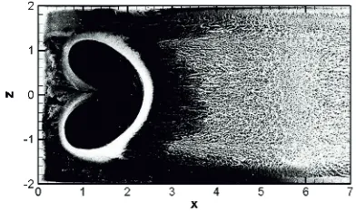
The flow over the backward facing step is considered to be 2D in sense of statistical characteristics as a rule, meaning that the ratio of the step height and channel width is very high, say more than 20. Then the flow-field in the middle third channel width is pretty 2D, with constant statistical characteristics along the span. Detailed study of the flow in a narrow channel, when the channel width / step height is lower than 10 is practically missing in public sources. The flow-field structure model in the recirculation region behind a step in narrow channel was suggested in [2]. The flow visualization on the channel bottom just behind the step showed a kidney-shaped region, suggesting existence of recirculation vortices impinging perpendicularly to the bottom.

The case has been studied in more details. The first publications [2,4] cover especially the mean flow structure, those results have been summarized in [6]. Then, the dynamical behaviour of the flow-field is studied in details. Information on dynamics of secondary

structures in prismatic channel of rectangular cross-section is in [3]. Then some studies on flow in channel with backward facing step have been carried out. Analysis of velocity field dynamical behaviour in a few planes perpendicular to the mean flow has been presented in [7].

The time-mean flow structure behind the step could be characterized by wall-shear distribution on the channel bottom. In Figure 1 the channel bottom is shown with result of the surface visualization using painting, published in [2]. Flow direction is from left in x direction, step edge position is x=0.

Figure 1. Surface visualization on the channel bottom.

The kidney pattern showed up just behind the step, and then back-flow region is located with distinct influence of secondary structures close to the channel walls. The reattachment process could be located in the region for

(

5.5, 6.2

)

x∈ , at least close to the channel axis.

The presented papers goal is to contribute to explanation of mechanisms behind creation of the kidney structure. It is focused on experimental confirmation of

C

Owned by the authors, published by EDP Sciences, 2014

existence of vortical structures impinging on the wall and description of theirs dynamical behaviour. This issue has not been addressed in available literature yet.

2 Experiment Setup

The existing blow-down test rig was modified for experiments with the separated flow in a channel with a backward facing step.

The tunnel has rectangular cross-section with filled corners within the contraction (to suppress corner vortices), honeycomb and a system of damping screens followed by contraction with contraction ratio 16. The area of the test section input is 0.25 m in height and 0.1 m in width. The time mean velocity departures from homogeneity in planes perpendicular to the tunnel axis are of order tenth of per cent with the exception of corners, where corner vortex starters could be detected. Conventional thickness of boundary layer at the step tip was approximately 4 mm. The natural turbulence level was about 0.1 % in the working section input. The channel downstream the backward facing step was 1 m in length

The step is placed close to the channel inlet with height h=25mm, the ratio of the input channel width to the step height was 4.

3 Experimental Techniques and

Evaluation Procedures

The same model of channel with backward-facing step has been used for the presented dynamical experiments as in [2,4,6,7]. The flow conditions are also the same, the input velocity of about U_i =21 m/s have been used resulting in Reynolds number based on the step height 34 400.

3.1. Experimental Techniques

The time-resolved PIV method was used for the experiments. The measuring system DANTEC consists of a double-pulse laser with cylindrical optics and CCD camera. The software Dynamics Studio 3.4 was used for velocity-fields evaluation. Laser New Wave Pegasus Nd:YLF, double head, wavelength 527 nm, maximal frequency 10 kHz, a shot energy is 10 mJ for 1 kHz (corresponding power 10 W per head). Camera Phantom V711 has maximal resolution 1280 x 800 pixels and corresponding maximal frequency 3000 double-snaps per second. The presented experiments are intended to cover low-frequency dynamics offering good statistics of the behaviour. Thus, for the measurements, the frequency

100 Hz and 4000 double-snaps in sequence

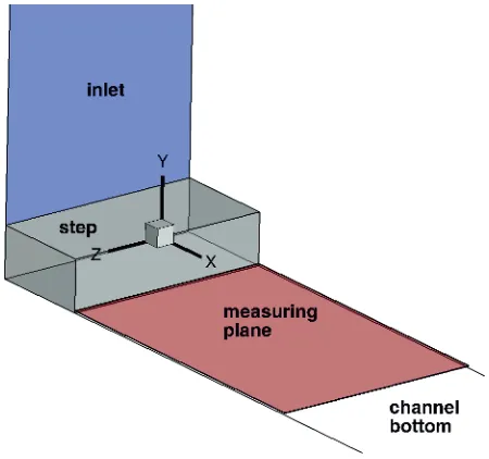
corresponding to 40 s of record for mean evaluation was acquired. The measuring plane was placed behind the step oriented parallel to the channel bottom in distance of about 1-2 mm above it – see Figure 2. Inlet section is shown in blue, measuring plane in red and the step is grey.

Figure 2. Schema of the experiment.

Please note the Cartesian coordinate system

(

x y z, ,

)

with x− axis in flow direction, y− perpendicular to the channel bottom and z− forming the step edge, its origin is placed in the middle of the step edge. All distances are non-dimensioned using the step height h (25 mm in the experiment). The measuring plane covers the channel width in z− direction and in x− direction starts on the step, being 6h long, thus it is defined in the following way:

( )

0; 6 , 0.94,

(

2; 2 .

)

x∈ y= − z∈ − (1)

3.2 Evaluation Procedures

The mean velocity field has been evaluated first to obtain the flow statistics and remove the mean flow. The dynamical behaviour was studied using the Oscillation Pattern Decomposition (OPD) method, which is described in details in [5].

The OPD method evaluates the basis representing oscillating modes of the extended dynamical system, which are characterized by a single frequency and damping representing cyclostationary elementary processes involved in the phenomenon notwithstanding that hidden. The structure can be typically a wave or travelling structures propagating in space, or pulsating pattern. Complex eigenvalue contains information on the cyclical phenomenon frequency and decay in time.

Navier-Stokes equation is modelled by Langevin equation for the linear Markov process:

( )

_{( ) ( )}

d t

t t

dt = ⋅ + u

B u ȟ (2)

where u

( )

t is vector of velocity fluctuations, B is the deterministic feedback matrix, ȟ

( )

t is noise driving the system which can be interpreted as influence of smaller, unresolved scales.

The eigenvalues βk of the feedback matrix B could

be related to the k-th mode dynamics, characterized by e-folding time τek and oscillation frequency fk as

follows:

( )

( )

Im 1 ; Re 2 k ek k k f β τ β π

= − = (3)

The eigenvalue characterizing each mode defines frequency and e-folding time. The frequency has obvious physical meaning. The e-folding time (or e-fold) is an appropriate measure of oscillatory process decay. The e-folding time is defined as the time required for the amplitude of an oscillation to decrease by a factor of e. The bigger e-folding time is, the smaller damping and the longer lasting process.

The corresponding complex eigenvector vk reveal

the mode topology. Contribution of the k-th OPD mode to the global dynamical process Vk

( )

t is given by the

following equation:

( )

ek cos 2

(

)

sin 2

(

)

t

k t e rk f tk ik f tk

τ _{π π}

−

= ª_¬ − º_¼

V v v , (4)

where vrk,vik are real and imaginary parts respectively

of the k-th OPD topology mode. The geometric and physical meaning of (4) is that between the spatial patterns vrk and vik the trajectory V

( )

t performs a

spiral with period T_k =1 f_k and e-fold time τe, in the

consecutive order

...

rk → ik → − rk → − ik →

v v v v (5)

repeating to infinity with amplitude decaying as

(

)

exp −tτ_ek .

The OPD method applies whitening procedure to the input data to solve the numerical issues. This procedure allows substantial reduction of the problems order and as a bonus the noisy components can be excluded from the analysis.

In general all OPD modes should be more or less damped (e-folding time is positive) in statistical sense described above. The growing feature (negative e-folding time) cannot be observed if statistics is performed properly. The unstable behaviour with negative e-folding time can be evaluated only if the signal record is too short to provide proper statistics and the corresponding pattern

is permanently growing during all the record by coincidence.

Periodicity p of a given mode could be introduced as e-folding time τe and oscillation period T ratio:

e e

p=τ T =τ f . (6)

The OPD modes are oscillating by definition. We could define non-oscillating uniformly decaying modes as such that decay too rapidly, with the periodicity p “too small”.

The spatial OPD modes consist of the real and imaginary parts respectively forming complex form. Two basic types of modes are possible as the complex structure regards. If the real part of the given mode is dominant while imaginary is very weak or even vanishing, the structures dynamics is of pulsating character. For traveling modes both parts are very similar with distinct structures, however shifted in space representing their positions in different phases of the cyclostationary decaying process (shift π 2). The speed

v of traveling structures could be estimated

v=s T=s f, (7)

where s is structures spacing and T is period.

5 Results

The measuring plane is located sufficiently close to the channel bottom (about 1-2 mm), the values of in-plane velocities characterize more or less the skin friction on the wall, if we suppose the velocity profile close to linear in this position.

The records of instantaneous velocity fields acquired in the measuring plane just behind the step are analysed. First, mean picture is evaluated, and then dynamical features are shown.

5.1 Time-Mean Results

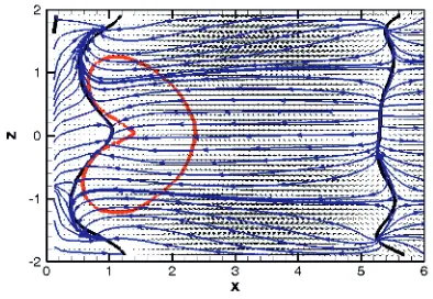
The time-mean velocity fields are to be presented first. The mean velocity vector-field in the measuring plane defined above is shown in Figure 3.

In Figure 3 the vector lines are added in blue, in red the contour of the kidney structure is given. The black lines represent the position of vanishing longitudinal mean velocity component U , dividing the area into parts with forward (U>0) and backward (U<0) mean flow. Note that between the black lines in the figure middle the back-flow region is located. Forward flow direction close to the step for 0< <x 1 is connected with appearance the tertiary vortex, while secondary vortex generates back-flow close to the bottom. To illustrate this, in Figure 4 there is mean velocity field in the plane of symmetry

0

z= .

Figure 4. Vectorlines of mean velocity field in the plane of symmetry.

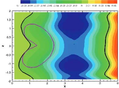
The distribution of the mean longitudinal velocity component is shown in Figure 5, while distribution of sum of variances in x and z directions is in Figure 6. In both figures the contour of the kidney region and U =0 lines are shown. The velocities are normalized using the velocity in the channel inlet.

Figure 5. Longitudinal velocity component distribution.

Figure 6. Sum of the in-plane velocity components variances.

The line of zero mean longitudinal velocity close to the step fits satisfactorily with the contour of the kidney region. The other zero line close to the position x=5.5 indicates the line of reattachment, however this is slightly shifted to the smaller x values (to the left) due to position of the measuring plane above the bottom and not exact on its surface. Confirm Figures 3-6 with the surface visualization in Figure 1.

The distribution of the longitudinal velocity component shows clearly the structure of the back-flow region close to the channel bottom. The minima of the mean longitudinal velocity (i.e. maximal back-flow) are located in position x=3.5 close to the middle of each channel half, z= ±1.

The distribution of the variances in Figure 6 shows that the fluctuating activity grows in the streamwise direction, maximum is located close to the plane of symmetry. However its value within the kidney region suggests that the velocity fluctuation even close to the bottom could reach more than 10 % of the inlet velocity.

5.2 Dynamics

For the dynamical analysis only part of the measuring plane was taken into account. We focused to the region adjacent to the step covering the kidney structure. The region of the measuring plane used for the OPD dynamical analysis is limited by x∈

(

0, 2.5

)

.

5.2.1 OPD Modes Overview

The OPD analysis was performed, the irrelevant noisy information dynamical content was filtered out. Minimal required autocorrelation coefficient value of time series characterizing the dynamical process involved was set to 0.3. This restriction results in 11 resolved OPD modes, the evaluated parameters are given in Table 1. The modes are ordered by descending e-folding time and thus importance.

Table 1. OPD modes.

Mode No.

f

[Hz]

e

τ

[ms]

p

[1]

St

[10-3]

1 8.18 37.67 0.308 9.436

2 6.85 24.56 0.168 7.905

3 11.14 23.28 0.259 12.853

4 0 16.01 0 0

5 3.92 15.36 0.060 4.524

6 3.62 9.15 0.033 4.176

7 8.08 8.93 0.072 9.317

8 6.87 7.05 0.048 7.920

9 0 6.41 0 0

10 16.17 5.08 0.082 18.653

The quantities given in Table 1 are the mode number, frequency in Hz, e-folding time in milliseconds, periodicity and Strouhal number respectively, for definitions see (3) and (6). The Strouhal number is evaluated in usual way using the mode frequency, inlet mean velocity and step height.

The modes frequency ranges from 0 to 16 Hz, however the maximal possible frequency covered by the experiment is given Nyquist frequency being half of the acquisition frequency and is 50 Hz. Maximal e-folding time for the evaluated modes is less than 40 ms suggesting that no really periodical process is involved. Strouhal numbers are relatively low, less than 0.02. The processes covered by the experiment are of really very low-frequency nature in this context.

In Figure 7 the spectrum is shown representing all 11 OPD modes in the plane frequency – e-folding time. In Figure 8 the periodicity values are represented graphically.

Figure 7. Spectrum of the OPD modes.

Figure 8. Periodicity parameter of the OPD modes.

The dominant 3 modes are those with biggest e-folding time and/or periodicity value. For the given case,

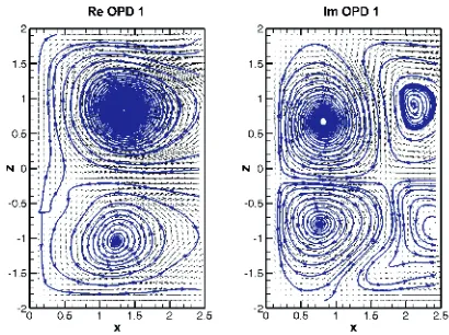
the modes 1, 2 and 3 could be considered as dominant. Topology of the dominant modes is shown in Figures 9, 10 and 11. The modes topology is descripted by vector fields of real and imaginary parts vrk and vik. To

visualize the structures involved (especially vortices), vector-lines (in blue) are added.

Figure 9. OPD mode 1 topology, real part v_r1 – left, imaginary part v_i1 – right.

Figure 10. OPD mode 2 topology, real part v_r2 – left, imaginary part v_i2 – right.

The dominant modes are oscillating with travelling character. Details are to be shown later in the separate chapter 5.2.2.

The modes 4, 9 and 11 are non-oscillating modes with zero frequency and thus vanishing imaginary part of the mode topology. As an example see topology of the mode No. 4 in Figure 12.

Figure 12. OPD mode 4 topology, real part v_r4 – left, imaginary part v_i4 – right (vanishes).

Dynamics of the non-oscillating modes consist in regular decay of the real part of the topological mode; the decay speed is defined by the e-folding time. The mode is of pulsating nature meaning that the structures do not move in space.

Modes 5, 6, 7 and 10 are characterized by very low value of the periodicity, less than 0.1, suggesting quick decaying nature. Those modes are typically of irregular, random type. As an example see Figure 13 showing the OPD mode 7 topology.

Figure 13. OPD mode 7 topology, real part v_r7 – left, imaginary part v_i7 – right.

Note that the OPD mode 7 is traveling, showing different topology in real and imaginary parts, however with approximately the same number of the vortical structures. Also note that the symmetry of this mode is broken completely.

5.2.2 Details on the Dominant OPD Modes

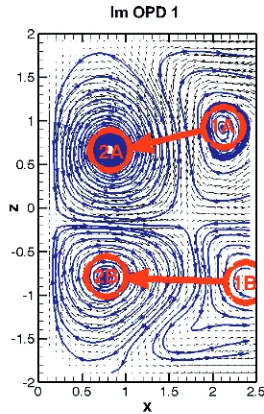
The dominant modes 1, 2 and 3 are characterized by the parameters and complex topological modes shown above. To follow the mode contribution in time, the formula (4) and (5) should be applied. From those follows that the same topology repeats each period and it is just opposite each half-period. We will demonstrate the given mode time evolution showing the imaginary part of the topological mode vik.

For the OPD mode 1, the imaginary part is in Figure 14, the cores of vortices are marked by circles in red with numbers.

Figure 14. OPD mode 1 dynamics.

In Figure 14 two pairs of contra-rotating vortices are captured, the first 1A, 1B, the second 2A, 2B. Note that vorticity of 2A and 1B is positive, while 1A and 2B is negative. A half period later, the topology will be the same, only signs of all vortices will be just opposite. This means that during the half-period (i.e. 61 ms) the vortex 1A moves into position 2A, while the vortex 1B into 2B, however keeping their sign.

Thus, the OPD mode 1 represents the train of

contra-rotating vortex pairs oriented in y direction with distance about 1.5 in z direction moving towards the step by the mean velocity v is 0.0146 of the inlet velocity

i

U , see (7). The vortex pairs appear periodically in trains changing theirs orientation on the regular basis during the single mode appearance.

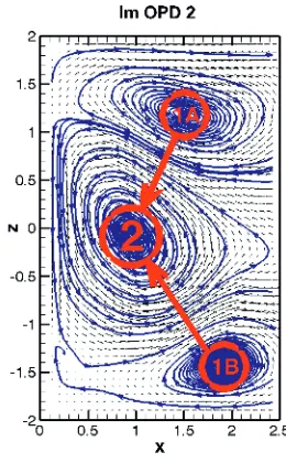
Thus, the OPD mode 2 represents coalescence of the

two co-rotating vortices into a single vortex of the same orientation.

Figure 15. OPD mode 2 dynamics.

The last dominant OPD mode 3 is shown in Figure 16. The mode could be interpreted as splitting of the single vortex 1 on the channel axis into two smaller vortices 2A and 2B moving towards the step corners by mean velocity of about 0.0133 Ui. The vortices cores are

just filling the kidney-shaped area, shown in green. Thus, the OPD mode 3 represents splitting of the

central vortex into two co-rotating vortices, all vortices of the same orientation.

Figure 16. OPD mode 3 dynamics.

The OPD mode 3 is the most probably directly connected with development of the kidney structure on the channel bottom, especially its downstream contour

(on the right-hand side). The contour close to the step is connected with the zero U line (confirm Figure 3).

6 Conclusions

Low-frequency dynamics of the recirculation zone behind the backward-facing step in narrow channel have been analysed in the presented paper using new experimental data.

The results suggest presence of several families of vortical structures with particular dynamics involving contra-rotating vortex pairs train, vortex splitting and coalescence.

Results offer explanation of creation mechanism of the kidney structure on the channel bottom.

7 Acknowledgement

This work was supported by the Grant Agency of the Czech Republic, project No. P101/10/1230.

References

1. Bradshaw, P. AGARD Conf. Proc.93 (1971)

2. Uruba, V., Jonáš, P., Mazur, O., International Journal of Heat and Fluid Flow 28 4 665–672 (2007)

3. Uruba, V.; Hladik, O.; Jonas, P., Journal of Physics Conference Series318 062021 (2011)

4. Uruba, V., Jonáš, P. Proceedings in Applied Mathematics and Mechanics. 12, 1, 501-502. (2012) 5. Uruba, V., EPJ Web of Conferences25 01095 (2012) 6. Uruba, V., Colloquium Fluid Dynamics 2012 IT

ASCR (Jonáš, P.; Uruba, V.) 33-34 (2012)