Optimization CBIR using
K-Means Clustering for Image Database
Juli Rejito*, Retantyo Wardoyo, Sri Hartati, Agus Harjoko
Department of Computer Science, Faculty of Mathematics and Science, Gadjah Mada University, Indonesia
Abstract— The CBIR (Content Based Image Retrieval) implementation in searching images into image database requires usually for a sufficiently prolonged time because such image searching process is performed with comparison between searched images and individually records in an image database. In this work, it is proposed a K-Means clustering algorithm aiming to develop clusters from each image database records, it can later be used for optimizing image searching access period. The stored images in image database records are only limited for the JPEG-type images. In this algorithm, cluster formation is based on maximum and minimum PSRN’s (Peak Signal to Noise Ratio) calculation values from individual records on a basic images and it will be treated as key images in every search for records with such cluster utilization. Results of the clustering process in form of cluster table would be made as indexing in early image searching for cluster position determination from searched images to image records.
Keywords— K-Means Clustering, CBIR, PSNR, Image Database
I. INTRODUCTION
Early in the 1990, CBIR, which conducted a retrieval process based on a visual content in a form of the compositions of image colors, began to be developed [1]. Currently, retrieval systems have also involved the user feedbacks, irrespective of whether or not an image of retrieval results was relevant (relevance feedback) which was used as a reference in modifying a retrieval process to obtain more accurate results [2].
Clustering is a method of grouping data objects into different groups, such that similar data objects belong to the same group and dissimilar data objects to different clusters [3]. Image clustering consists of two steps the former is feature extraction and second part is grouping. For each image in a database, a feature vector capturing certain essential properties of the image is computed and stored in a feature base. Clustering algorithm is applied over this extracted feature to form the group.
In Iyengar G. and Lippman A. the authors propose to use clustering techniques to allow for efficient access to large image databases [4]. More efficient access is important, since due to the size of large image databases, querying becomes expensive even if the images are represented in a compact manner. With clustering, the task of retrieval is decomposed into a two stage process. In the first step an appropriate cluster is selected and in the second step the best matches from this cluster are returned. They compare a clustering technique which uses relative entropy to techniques using the Euclidean
norm. Kaster T., et all. propose to use image clustering techniques to allow for faster searching in image databases. They compare different clustering techniques to find out which suits the task of clustering images best [5].
In Saux B. L. and Boujemaa N. the authors propose to use image clustering to give a good overview of an image database to help a user find a sought image faster.To cluster this images, they estimate the distribution of image categories and search the best representative for each cluster [6]. They represent images by a high-dimensional feature vector and propose a new clustering algorithm which they compare to other clustering techniques. In [7], [8], and [9] give general information about clustering of data and the evaluation of results. In [10] a new clustering algorithm based on the EM algorithm is proposed and a method to avoid the problem of finding an initial partition by iterative splitting of an initial Gaussian describing all data points is introduced.
The Peak Signal to Noise Ratio is the error criterions used to compare the M x N pixels image I loaded from the conventional JPEG format and the proposed image loaded from the MJPEG. Typical PSNR values range between 20 and 40. The actual value is not meaningful, but the comparison between two values for different reconstructed images gives one measure of quality. Several research groups are working on perceptual measures (for example [11], and [12]) and concluded that the traditional SNR measures do not equate with human subjective perception. Hence a higher value of PSNR is better for comparison of two images because it means that the ratio of Signal-to-Noise is higher. Therefore a compression scheme having a high PSNR is expected for evaluating the existing compression algorithm. In general, the higher PSNR value of an image implies the better image quality.
work, clustering process consist of three phase, namely, to make minimum and maximum PSNR value calculation, and the PNSR range from each image record, the second phase is to make cluster initialization, and finally is cluster formatting.
II. OBJECTIVE QUALITY MEASUREMENT
For objective estimate of the scaling algorithm’s quality is used the main approach in digital image processing, based on computing MSE and PSNR. MSE represents the average square error (difference) in the intensities and of a given color of the corresponding pixels from the both images and it is dimensionless quantity. Because of its simplicity, it is the most common method of objectively measuring image quality given a reference image
where Let M and N are dimensions of the images and are the to images to be compared.
PSNR represents the square of the ratio between the maximum of the signal (the maximal possible value of color’s intensity and the mean square error (difference) in the intensities and color of the corresponding pixels from the both images and is measured in decibels (dB)
The estimate can be done by computing MSE and PSNR for every single color (Red, Green, Blue), as well as totally for the three of them.
III.K-MEANS ALGORITHM
It is assumed that there were n clustered objects to get a sample set, that is, . By using K-means algorithm, n sample objects are grouped into K clusters to ensure the similarities among samples in the same cluster and the differences among samples in different clusters. Specific procedure is as follows:
1) Randomly select K objects as initial cluster centers as following:
2) According to the minimum distance principle, that is,
each sample object is assigned to one of K clusters
3) Take the average values of objects of each cluster as new clustering centers, average values can be get by
nj is the number of objects in the cluster j
4) If the cluster centers have changed, repeat 2), 3) steps until the cluster centers do not change. As a result, clustering criterion function can be converged
Cj is the clustering center of cluster Sj .
IV.PROPOSED WORK
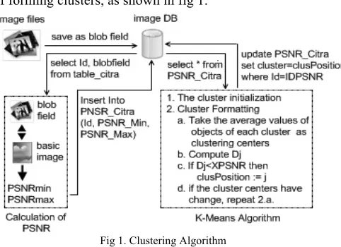
A clustering design refers to a clustering algorithm by using both minimum and maximum PSNR values as a basis of forming clusters, as shown in fig 1.
Fig 1. Clustering Algorithm
A. Calculation of the minimum and maximum PSNR values The record image ( ) can be calculated its PSNR values by comparing it with the basic image ( ) with condition that such two images have same pixel sizes. If those two compared pixel sizes vary, thus it must be made formerly a resizing process on either images and therefore the two images to be compared may have a same pixel sizes. The commonly used objective measure are (MSE Red), (MSE Green), (MSE Blue), , and
, which are calculated as
In this work, images are stored in an image table with blogfield attribute utilization and they have similar size, 512x512 pixels in 24 bits image in depth. The used basic image as key images for mapping media that will result in the PSNR value also have similar sizes and depth.
Algorithm 1 : Calculation of PSNRMin and PSNRMax Input : Blobfield from Table_Citra and Basic Image. Output : PSNR_Citra Table
1. I2 := Set initial Basic Image
2. Select Id, BlobField from Table_Citra 3. While not Table_Citra.EOF do begin 4. ImageID := Table_Citra.ID 5. I1 := Table_Citra.Blobfield
6. ComputePSNR(I1, I2)
7. Insert Into PNSR_Citra (Id, PSNR_Min, PSNR_Max) values (ImageID, PSNRMin, PSNRMax)
8. Next Record 9. End
Algorithm 2 : Compute PSNR
1. procedure ComputePSNRMin(Img1,Img2 : Tbitmap) 2. var R1,G1,B1,R2,G2,B2, i,j,pjg,lbr : integer
MSEx : array[1..3] of real col1,col2 : TColor
MSEMin, MSEMax, PSNRMin, PSNRMax : real 3. begin
4. MSEx[1] := 0.0;MSEx[2] := 0.0;MSEx[3] := 0.0 5. pjg := Img1.Bitmap.Width; lbr := Img1.Bitmap.height 6. for i := 0 to (pjg-1) do begin
7. for j := 0 to (lbr-1) do begin
8. col1 := Img1.Bitmap.Canvas.Pixels[i,j] 9. R1 := getRvalue(col1)
10. G1 := getGvalue(col1) 11. B1 := getBvalue(col1)
12. col2 := Img2.Bitmap.Canvas.Pixels[i,j] 13. R2 := getRvalue(col2)
14. G2 := getGvalue(col2) 15. B2 := getBvalue(col2)
16. MSEx[1] := MSEx[1]+((R1-R2)*(R1-R2)) 17. MSEx[2] := MSEx[2]+((G1-G2)*(G1-G2)) 18. MSEx[3] := MSEx[3]+((B1-B2)*(B1-B2)) 19. end;
20. end;
21. MSEx[1] := MSEx[1]/(pjg*lbr) 22. MSEx[2] := MSEx[2]/(pjg*lbr) 23. MSEx[3] := MSEx[3]/(pjg*lbr) 24. MSEMin := 100000.0; MSEMax := 0.0 25. for i := 1 to 3 do begin
26. if MSEMin>MSEx[i] then MSEMin := MSEx[i] 27. if MSEMax<MSEx[i] then MSEMax := MSEx[i] 28. end
29. PSNRMin := 10.0 * log10((255.0*255.0)/MSEMax) 30. PSNRMax := 10.0 * log10((255.0*255.0)/MSEMin) 31. End
B. The Cluster Initialization
The cluster formatting phase was begun with an early initialization in individual clusters before it is made grouping for those records into their respective clusters. An early initialization for each clusters may be formatted by its PSNR_Min values produced in first algorithm in PSNR
Table_Citra table, and then it would be treated as basis for record sequence. Furthermore, it is specified distance between clusters by counting total records and divided with total clusters and it is finalized by determining every taken cluster up from successive records in accordance with changes in distance. This early initialization algorithm is written as follow:
Algorithm 3 : Set Initial Centroids Input : k // Numbered of clusters
Select PSNRMin, PSNRMax from PSNR_Citra Output : Centroid
1. k := Set Input Cluster Count 2. Centroid := array[1..k,1..2] of real
3. Select id, PSNR_Min, PSNR_Max from PSNR_Citra Order By PSNR_Min
4. xDistance := RecordCount DIV k 5. For i:=1 to k do Begin
6. RecID := PSNR_Citra.Id
7. Update PSNR_Citra set Cluster= i where ID=RecID
8. PSNR_Citra.moveby(xDistance) 9. End
C. Cluster Formatting
After an early initialization is made for individual cluster, so this centroid would be used as starting center point for each clusters, so that every records will be given adjustment in their respective cluster position by counting formerly distance of image record to nearest cluster by using this Euclidean’s distance formula :
where Dj is the Distance
is Minimum Centroid j-th cluster is Maximum Centroid j-th cluster
A distance, Dj calculation is performed by counting total
quadrate from differences in minimum PSNR values with the j-th minimum clustering center added by maximum PSNR value with the j-th maximum clustering center. Its product would then be made into quadrate and it will produce required distance. The nearest distance one to intended cluster is also given a recalculation for obtaining value from such clustering center. This process will be repeated again on initial record from such image database up to clustering center will not perceive a change anymore.
Algorithm 4 : Cluster Formatting
Input : a set of record and number of cluster Output : K-Centroid and members of each cluster 1. Set Initial Centroids (Algorithm 2)
2. Selesai := true 3. While Selesai do begin
4. Xquery := select Cluster, avg(PNSRMin) as Xmin, avg(PSNRMax) as Xmax From PSNR_Citra group by Cluster
5. While not Xquery.EOF() do begin 6. Centroid(Xquery.Cluster,1):=Xquery.XMin 7. Centroid(Xquery.Cluster,2):=Xquery.XMax 8. Xquery.next
9. End
10. PSNR_Citra.first
11. While not PSNR_Citra.EOF do begin 12. IDPSNR := PSNR_Citra.Id
13. ClusCurrent := PSNR_Citra.Cluster 14. ClusPosition := 1; XPSNR := centroid(1,1) 15. for j:=1 to k do begin
16. Compute Dj
17. If Dj < XPSNR then ClusPosition := j
18. End
19. Update PSNR_Citra set Cluster=ClusPosition where PSNR_Citra.Id=IDPSNR
20. If ClusPosition<>ClusCurrent then Selesai := true else Selesai := false
21. PSNR_Citra.next 22. end
23. end
V. IMPLEMENTATION AND EXPERIMENTAL RESULTS This algorithm implementation is made by using 4,000 files of the JPEG-typical images in 512x512 pixel sizes with 24 bits in depth and it is stored as an image record in image table by using a blob field-type attribute. The image record in such Image Record is furthermore known as process from those three above algorithms, and then it would be developed clusters in various testing groups. Table I shows product of minimum and maximum PSNR values for 10 initial records as sample of records from 4,000 records after it was made a mapping on basic images.
TABLE I
SAMPLE OF RECORDS
Image RecordID PSNRMin PSNRMax
Image RecordID PSNRMin PSNRMax
(1).jpg 1.765565 9.664234
00309.jpg 12.718576 13.060186
(2).jpg 3.618844 7.217159
00322.jpg 7.791683 19.702308
00011_0.jpg 8.268525 11.896743
00325.jpg 5.643815 13.019012
0002-1.jpg 2.511891 7.581959
00335.jpg 11.771915 12.884302
0009-1.jpg 4.879889 7.600446
00386.jpg 10.521531 13.082261
The implementation of the clustering was applied in several cluster groups, namely, 2 clusters, 4 clusters, and 8 clusters, and the amounts of iteration of each cluster and the values of minimum Centroid and maximum Centroid for each cluster were shown in Table II.
TABLE II
CLUSTERING OF 4,000IMAGE DATABASE RECORDS IN 2,4, AND 8
CLUSTERS
Cluster
group Number of cluster
Cluster Centers Record Count PSNRMin PSNRMax
2 1 7.3248 12.4807 2406
2 2 3.0613 7.7925 1594
4 1 5.6727 12.5336 933
4 2 2.1925 6.3712 803
4 3 4.6237 9.4844 1161
4 4 9.1404 13.2625 1103
8 1 6.1977 11.5169 604
8 2 1.8016 5.6546 462
8 3 3.0334 7.8349 629
8 4 4.8183 9.6886 674
8 5 3.7400 13.1370 304
8 6 8.3888 11.1569 555
8 7 7.9600 15.3997 434
8 8 10.4274 13.4723 338
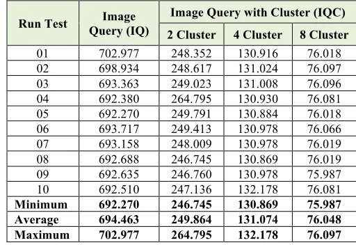
Table III shows in detail the results of testing process by using image query and that of image query with cluster by using 4,000 records stored in an image database. The testing was conducted 10 times by using different searching base images. From the testing of query, a average time of 694.463 ms (millisecond) was obtained, whereas from the testing of image query by using cluster for each cluster a average time of 249.864 ms, 131.074 ms, and 76.048 ms for 2, 4, and 8 clusters, respectively, were obtained.
TABLE III
THE RESULTS OF ACCESS TIME TESTING OF 4,000
IMAGE DATABASE RECORDS BY USING IMAGE QUERY AND
IMAGE QUERY WITH CLUSTER
Run Test Query (IQ) Image Image Query with Cluster (IQC) 2 Cluster 4 Cluster 8 Cluster
01 702.977 248.352 130.916 76.018 02 698.934 248.617 131.024 76.097 03 693.363 249.023 131.008 76.096 04 692.380 264.795 130.930 76.081 05 692.270 249.791 130.884 76.018 06 693.717 249.413 130.978 76.066 07 693.158 248.009 130.978 76.019 08 692.688 246.745 130.869 76.019 09 692.635 246.760 130.978 75.987 10 692.510 247.136 132.178 76.081
Minimum 692.270 246.745 130.869 75.987 Average 694.463 249.864 131.074 76.048 Maximum 702.977 264.795 132.178 76.097
TABLE IV
THE RESULTS OF ACCESS TIME RATIO
IMAGE QUERY AND IMAGE QUERY WITH CLUSTER
Run Test Ratio of Access Time IQ : IQC 2 Cluster 4 Cluster 8 Cluster
01 2.831 5.370 9.248
02 2.811 5.334 9.185
03 2.784 5.293 9.112
04 2.615 5.288 9.101
05 2.771 5.289 9.107
06 2.781 5.296 9.120
07 2.795 5.292 9.118
08 2.807 5.293 9.112
09 2.807 5.288 9.115
10 2.802 5.239 9.102
Minimum 2.615 5.239 9.101
Average 2.781 5.298 9.132
Maximum 2.831 5.370 9.248
A comparison of the access times of image query and image query with cluster showed that the greater the size of formed cluster, the higher the speed of needed access time. The ratio of average time access of image query to image query with cluster for 2 clusters was 2.781 or, in the other words, there was an increase of access time by 2.781 when the access used 2 clusters as compared to that of image query. For 4 and 8 clusters there occurred an increase of access time by averagely 5.298 times and 9.132 times, respectively.
VI.CONCLUSION
1. The image database record clustering used in this research was conducted based on the computation of minimum and maximum PSNR values of each image database record by using basic image.
2. The results of 10 times of testing on image query in image database by using records that was taken randomly by an amount of 4,000 showed that the average access time was 694.463 ms. The results of testing by using image query
with cluster for 2, 4, and 8 clusters were 249.864 ms, 131.074 ms, and 76.048 ms, respectively.
3. The ratio of the access time of image query to image query with cluster by using 2, 4, and 8 clusters showed significant increases in access time, that is, 3 times, 5 times, and 9 times for 2, 4, and 8 clusters, respectively.
REFERENCES
[1] Remco, C.V., Mirela, T., “Content-based image retrieval systems: a survey”. Tech. Report, Department of Computing Science, Utrecht University, 2000.
[2] Long, F., Zhang, H., and Feng, D., “Fundamentals of content-based image retrieval”. In Feng, D., Siu, W. C., and Zhang, H. J., (eds.), Multimedia Information Retrieval and Management – Technological Fundamentals and Applications. Springer, 2002. [3] Han, J., Kamber M., “Data Mining: Concepts and Techniques”.
Morgan Kaufmann Publishers, 2nd Edn., New Delhi, ISBN: 978-81-312-0535-8, 2006.
[4] Iyengar G., Lippman A. “Clustering Images Using Relative Entropy for Efficient Retrieval”. Proc. Workshop on Very Low bitrate Video Coding, Urbana, IL. 1998.
[5] K¨aster T., Wendt V., G. Sagerer. “Comparing Clustering Methods for Database Categorization in Image Retrieval”. Proc. DAGM 2003, Pattern Recognition, 25th DAGM Symposium, Vol. 2781 of Lecture Notes in Computer Science, pp. 228–235, Magdeburg, Germany, 2003.
[6] Saux B. L., Boujemaa N. “Unsupervised Robust Clustering for Image Database Categorization”. Proc. International Conference on Pattern Recognition, Vol. 1, pp. 259–263, 2002.
[7] Berkhin P. “Survey of Clustering Data Mining Techniques”. Technical report, Accrue Software, San Jose, CA, 2002
[8] Jain, A.K., Dubes R.C., “Algorithms for Clustering Data”. Prentice Hall Inc., Englewood Cliffs, New Jersey, ISBN: 0-13-022278-X, pp: 320,1988.
[9] Jain A. K., Murty M. N., Flynn P. J. “Data Clustering: A Review. ACM Computing Surveys”, Vol. 31, No. 3, pp. 264–323, 1999. [10] Linde Y., Buzo A., Gray R.. “An Algorithm for Vector
Quantization Design”. Proc. IEEE Transaction
Communications,Vol.28,pp.84–95, 1980.
[11] Netravali A.N., Haskell B.G.,”Digital Pictures: Representation, Compression, and Standards”, (2nd Ed), Plenum Press, New York, NY., 1995.
[12] Rabbani M., Jones P.W., “Digital Image Compression Techniques”, Vol TT7, SPIE Optical Engineering Press, Bellvue, Washington,1991