Event Generators for Multi Hadronic Production in
e
+e
−Colli-sions
Rong-Gang Ping1,2,⋆and Zhen Gao3,⋆⋆
1Institute of High Energy Physics, Beijing 100049, People’s Republic of China
2University of Chinese Academy of Sciences, Beijing 100049, People’s Republic of China
3University of Science and Technology of China, Hefei 230026, China
Abstract. An event generator for multi hadron production is presented for measuring the R value in theτ-charm energy region with e+e− collisions. The initial state radiation effects are considered up to second order accuracy, and the radiative correction factor is calculated with hadronic Born cross sections. The established exclusive processes are generated according to their measured cross sections, while the missing processes are generated using the LUND Area Law model, and its parameters are tuned with data collected at √s =3.08 GeV. The optimized values are validated with data in the range √
s=2.2324∼3.671 GeV. These optimized parameters are universally valid for event generation below the D ¯D threshold.
1 Introduction
The total cross section for multi hadron production in positron-electron (e+e−) annihilation is one of
the most fundamental observables in particle physics. A precise measurement of the hadronic cross section allows us to determine the hadronic contributions to the running of the quantum electrody-namic (QED) fine structure constantα, electroweak parameters, and the strong couplingαs. The R value, defined as the ratio of the total hadronic cross section to that of e+e− → µ+µ−at Born level,
have been measured by many collaborations in e+e−scan experiments, over the center-of-mass energy
from the two pion mass threshold (M2π) to the Z peak [1]. In the tau-charm energy region, the R values
measured at BESII [2] were used in the evaluation of the hadronic contribution from the five quark loops at the energy of Z peak,∆α(5)had(MZ2), with an improved precision by a factor of 2 [3].
A large number of exclusive processes have been measured over the range from M2πto 5 GeV [4],
but most cross sections have large uncertainties. To improve these measurements, a hadronic event generator is needed for us to get better understanding of background events from e+e−→hadrons.
Especially, a precise R-value measurement requires excellent control of radiative correction (RC) and vacuum polarization (VP) in the Monte Carlo (MC) program. We design an event generator for measuring R values and exclusive decays in e+e−collisions. The generator is constructed in the
framework of BesEvtGen [5], incorporating both the RC and VP effects. We also present details of the parameter optimization of the Lund Area Law (LUARLW) model [6] with data, and validations with various distributions within the energy range √s=2.2324∼3.671 GeV.
2 Framework of event generator
The generator is constructed as a model of the BesEvtGen package. It provides the 4-momentum of each final state particle for detector simulation, and provides the ISR correction factor and VP factors for users to undress the observed cross section. The basic idea of this generator is to decompose the total hadronic cross section into the measured exclusive processes and remaining unknown processes. The latter are generated with theLUARLWmodel.
2.1 Initial state radiative correction
e−
e+
Xi
e−
e+
Xi
γ
(a) (b)
Figure 1. Feynman diagrams for the process (a) e+e−→Xi, and ISR process (b) e+e−→γISRXi.
In an e+e−energy scan experiment, we consider a measurement of the Born cross section (σ0) for
a process e+e−→Xi, as shown in Fig. 1 (a), where Xidenotes the hadron states of i-th process. Due
to ISR, the observed cross section (σ) is actually for the process e+e−→ γISRXi, as shown in Fig. 1 (b). The observed cross section is related to the Born cross section by the quasi-real electron method [7]:
σ(s)=
Z √s
Mth dm2m
s W(s,x)
σ0(m)
|1−π(m)|2, (1)
where m is the invariant mass of the final states;π(m) is the vacuum polarization function, which will be discussed later; s is the e+e−center-of-mass energy squared; x≡2Eγ∗/
√
s=1−m2/s, and E∗γis
the total energy carried by ISR photons in the e+e−center-of-mass frame; Mthis the mass threshold of a given process. W(s,x) is a radiative function, we use the result of QED calculation up to orderα2 [8].
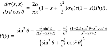
At the leading order of QED calculation, the ISR photon is characterized by soft energy and beam collinear distribution. A more general result is obtained by the method of Bonneau and Martin[11] up to m2
e/s terms, and the angular distributions is calculated by
dσ(s,x) dxd cosθ =
2α
πx(1−x+ x2
2)σ0(s(1−x))P(θ), (2)
with
P(θ)=
sin2θ−2(xx22−sin2x4+θ2)−
m2 e
E2
(1−2x) sin2θ−x2cos4θ
x2−2x+2
sin2θ+m2e
E2cos2θ
2
, (3)
2.2 Vacuum polarization
The vacuum polarization (VP) has been calculated by many groups and is available in the literature. Comparisons between them are given in Ref. [12]. There are notable differences below 1.6 GeV, and above 2.0 GeV; visible differences appear when approaching the charmonium resonances. We use the results from the Fred Jegerlehner group [13]. It provides leptonic and hadronic VPs both in the space-and time-like region. For the leptonic VP the complete one- space-and two-loop results space-and the known high-energy approximation for the three-loop corrections are included. The hadronic contributions are given in tabulated form in the subroutine HADR5N [14].
2.3 Cross sections for exclusive processes
We collect 25 exclusive modes, e+e− → ΣΣ¯0 [16], ΛΣ¯0 [16], Σ0Λ¯ [16], K+K−π0 [18] , KSK+π−
[18] , KSK−π+ [18], K+K−η [18], K+K−2π0 [21], 2(K+K−) [22], 2(π+π−)π0 [23], 2(π+π−)η
[23], K+K−π+π−π0 [23] , 3(π+π−) [24], 2(π+π−π0) [24], K∗(892)0K+π− [21], K∗(892)0K−π+ [21],
K∗
2(1430)
0K+π−[21] , K∗
2(1430)
0K−π+[21], K+K−ρ0 [21],φπ+π−[21],η′π+π−[16],Σ−Σ¯+[16],ωη
[24] andφη′, with energy region covering from 0.3 GeV up to about 6 GeV. Events of these modes are
generated with model ConExc [25]. Events for other ten exclusive modes are generated the generator model PHOKHARA [26], ie. e+e− → p ¯p, n ¯n,ΛΛ,¯ π+π−,π+π−2π0, 2(π+π−),π+π−π0, K+K−, KSKL
andπ+π−ηprocesses.
The narrow vector resonances, such asψ(3770), ψ(2S ), J/ψ, ρ(1700), and ω(1420), are also in-cluded in the calculation for the ISR correction factor. The cross sections for these narrow resonances are represented with the Breit-Wigner function
σBW(s)=12π
γeeγ (s−M2)+M2γ2,
where M, γ,andγeeare the mass, total width and partial decay width to e+e−final state, respectively. The distribution of cross section versus center-of-mass energy is described by an empirical func-tion, which is parameterized with a multi-Gaussian function. Its parameters are determined by fitting the cross section mode by mode. These empirical functions are used in the generator for the calcula-tion of the ISR correccalcula-tion factor and event type sampling.
The angular distribution for ISR photons is implemented according to Eq. (2). However, angular distributions are implemented only for two-body decays, namely, 1−cos2θ for PP (where P is a pseudoscalar meson) modes, and 1+αcos2θfor the PV (α=1) and B ¯B modes, where V is a vector meson, and B is a baryon. The angular distribution parameterαfor the B ¯B mode is taken as the quark
model prediction [27]. The phase space model is used for multi-body decays.
2.4 LUND Area Law model
The hadronic events produced in the e+e− annihilation are evolved as follows. As the first step, a
quark-antiquark (q ¯q) pair is produced from a virtual photon, coupled to the e+e− pair. Then the q ¯q branching proceeds via emitting gluons, and further develops into hadrons. In the high energy
In the tau-charm energy region, theLUARLWmodel [6] has been proposed to estimate the mul-tiplicity distribution for primary hadrons produced from the string fragmentation. The probability distribution reads:
Pn=
µn
n!exp[c0+c1(n−µ)+c2(n−µ)
2], (4)
withµ = α+βexp(γ√s), where c0,c1,c2, α, β andγ are parameters to be tuned with data. An interface to access theLUARLWmodel is designed in the BesEvtGen [5] framework, and is only used to generate the primary hadrons. The further decays into light hadrons are realized with BesEvtGen [5].
2.5 Monte Carlo algorithm
The event sampling proceeds via two steps. Firstly, the mass of the hadron system, Mhadrons, is sampled according to the distribution of the observed cross section, i.e. dσ(s)/dm, for the process e+e−→γIS RXiaccording to Eq. (1). For simplicity, the ISR energy, √s−Mhadrons, is imposed on
a single photon. The second step is to sample the event type topology according to the ratios of individual cross sections at the energy point Mhadrons.
2.5.1 Sampling ofMhadrons
To sample the Mhadrons, we split the region Mth ∼ √s into a few hundred intervals. The cumulative
cross section up to the i-th interval, mi, is
ˆ
σ(mi)= 1
σ(s)
Z mi
Mth dm2m
s W(s,x)
σ0(m) |1−π(m)|2.
The Mhadronsis sampled according to the ˆσ(mi) distribution with the discrete MC sampling technique.
2.5.2 Sampling of event type
Using the discrete MC sampling technique, the final states for exclusive modes are sampled according to the ratios of their cross sections (σm) to the total cross section (σtot), i.e.,
cm=σm(Mhadrons)/σtot(Mhadrons),
where m is an index for exclusive precess, and events for the remainder part, 1−P
mcm, are generated with theLUARLWmodel.
3 Optimization of
LUARLWparameters
3.1 Strategy to optimize theLUARLWparameters
An ensemble of MC samples was produced within the framework of the BesEvtGen [5] event generator, and then it is subject to detector simulation with BOSS software [40]. 91 independent MC samples were prepared, each one generated with a different set ofLUARLWparameters, which were randomly chosen in the parameter space around a given central point p0. All MC samples were produced with equal statistics, and were large enough so that the overall statistical uncertainties are negligible.
By including the correlations among the model parameters, the dependence of physical observable is expanded up to the quadratic term as done in Ref. [37], and the response function reads
f (p0+δp,x)=a (0) 0 (x)+
n
X
i=1
a(1)i (x)δpi
+ n
X
i=1 n
X
j=i
a(2)i j (x)δpiδpj≈MC(p0+δp,x), (5)
where n is the number of parameters to be fitted, and MC(p0 +δp,x) denotes the distribution of
physical observable x predicted for a given set of parameter values p0+δp, where p0is the central value andδpiis the deviation of the i-th parameter. The quadratic term in the expansion accounts for the possible correlations between the model parameters. The number of coefficients a(0,1,2), L, in the expansion is calculated with
L=1+n+n(n+1)/2, (6)
and the coefficients are determined by fitting Eq. (5) to the L reference simulation distributions. This fit is equivalent to solving a system of linear equations of Eq. (5). Then the optimal values of the parameters pi, their errorsσi, and their correlation coefficientsρi jwill be determined with a standard
χ2fit to data using packageMINUIT[38]. The fit is done simultaneously for all distributions and for all bins.
To minimize statistical uncertainties, the model parameters should be fitted to the distributions that show strong dependence on the parameters under consideration and least dependence on the others. For each distribution, a quality to measure the sensitivity to the model i-th parameter is calculated, i.e.
Si(x)= δMC(x)
MC(x) pi
.δpi
pi ≈
∂ln MC(x)
∂ln|pi|
pi
, (7)
whereδMC(x) is the change of the distribution MC(x) when the model parameter piis changed by
δpi from its central value. Sensitivity values for charged track distributions and event shapes vary within the range from -0.3 to 0.3, but the polar angle and azimuthal distributions for charged tracks are not sensitive to the change of model parameters. This is because the inclusive charged tracks are distributed isotropically over the whole phase space. Taking the sensitivity into consideration, only 12 observable distributions are kept for the model parameter fit. They are the number of photons (Nγ),
the number of charged tracks (Ntrack), momentum of tracks (Ptrack), xf = 2Pz/W, x⊥ = 2P⊥/2W, sphericity, aplanarity, thrust, oblateness, and Fox-Wolfram moments (H20,H30,H40) [29], where W is the total reconstructed energy of an event, and P⊥is the transverse momentum.
We have 12 parameters to be optimized. According to Eq. (6), there are 91 coefficients, a(0,1,2) in Eq. (5) to be determined. Hence we need at least 91 MC samples to determine these coefficients. These were prepared with 0.5 million events for each sample. Then the dependence of response func-tion on model parameters is established, and this analytical expression is used to simultaneously fit to the data distributions after QED background events are subtracted. In the optimization procedure, the
χ2function is defined over each bin, ie.,χ2
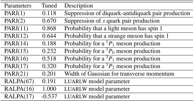
Table 1. Optimized parameters at √s=3.08 GeV. The statistical errors are negligible.(2S+1)P
Jdenotes a meson
has spin S , orbital angular momentum (L) and total spin J.
Parameters Tuned Description
PARJ(1) 0.118 Suppression of diquark-antidiquark pair production PARJ(2) 0.670 Suppression of s quark pair production
PARJ(11) 0.868 Probability that a light meson has spin 1 PARJ(12) 0.644 Probability that a strange meson has spin 1 PARJ(14) 0.188 Probability for a1P
1meson production PARJ(15) 0.232 Probability for a3P0meson production PARJ(16) 0.518 Probability for a3P
1meson production PARJ(17) 0.320 Probability for a3P2meson production PARJ(21) 0.201 Width of Gaussian for transverse momentum RALPA(67) 0.191 LUARLWmodel parameter
RALPA(16) 1.000 LUARLWmodel parameter RALPA(17) -0.537 LUARLWmodel parameter
bins. To consider the requirement of fit goodness on the multiplicity of charged tracks, this distribu-tion is weighted with a factor of 10, while other distribudistribu-tions are weighted with a unitary factor. This weighted factor is chosen by requiring that the fit quality of all distributions are satisfactory.
3.2 Event selection and fit results
We use the data taken at √s=3.08 GeV to optimize the parameters. To validate the parameters, we compare the MC distributions to the data distribution within the energy region 2.0 – 4.26 GeV. The QED backgrounds, e.g. e+e− →e+e−, γγ, γ∗γ∗, µ+µ−, andτ+τ−are subtracted using MC samples,
and they are normalized according to their cross sections to the luminosity of data sets. The event selection criteria for light hadrons are similar to those applied to the R value measurements [2, 39].
The selected candidates are characterized by the distributions of charged track multiplicity (Ntrack), track energy (Etrack) and momentum (ptrack), polar angle (cosθ), azimuthal angle (φ), rapidity, peseu-dorapidity, and a set of event shapes. These distributions are normalized to one and the errors are scaled for all bins.
To consider the possible correlations between these observable quantities, different observable combinations were tried. In each combination, track observables, Nγ, Ntrack, Etrack, xf and x⊥, must
be included, while the ptrackdistribution or event shapes are partly included in the simultaneous fit. Generally speaking, the more observable distributions are involved in the fit, the worse fit quality one gets. To validate the resulted parameters, they are reused to generate MC samples, and compared to data.
4 Validation of tuned parameters
To select the most optimal values, we compare the data to the MC distributions, which are generated with optimized parameters for all sets. We require that the parameters can produce MC distributions having the best fit goodness qualityχ2/N, where N is the total number of bins for calculating theχ2
To validate this set of parameters for the MC generation below the D ¯D threshold, we compare
the multiplicity distributions for charged tracks at 14 energy points from√s=2.2324 to 3.671 GeV, as shown in Fig. 2. When extending these parameters from 3.65 GeV to low energy points, the agreement between the data and MC gets better. This is due to the fact that the total cross section equals the sum of the exclusive ones when approaching the energy 2.0 GeV.
5 Discussion and summary
To summarize, we have developed an event generator for R measurement at energy scan experiments, incorporating the initial state radiation effects up to the second order correction. The ISR correction factor is calculated using the measured Born cross sections. The established exclusive processes are generated according to their measured cross sections, while missing processes are generated using the LUARLWmodel, with tuned parameters at 3.08 GeV. To validate the optimized parameters, various MC distributions are compared to the data distributions with data from energy √s=2.2324 to 3.671 GeV. We conclude that the optimized parameters are valid for MC generation below the D ¯D threshold.
Above the D ¯D threshold, the parameters should be optimized with the charm meson decays.
Acknowledgements: The work is partly supported by the National Natural Science Foundation of China under Grants Nos. 11645002, 11375205, and 11565006.
References
[1] For the most recent reviews, see, for example, B. Pietrzyk, Nucl. Phys. B (Pro. Suppl.), 162, 18 (2006); F. Jegerlehner, Nucl. Phys. B (Pro. Suppl.), 162,22, (2006) [hep-ph/0608329]; F. Am-brosino et al, Eur. Phys. J. C, 50, 729 (2007) [hep-ex/0603056].
[2] J. Z. Bai et al(BES Collaboration), Phy. Rev. Lett. 88, 101802 (2002) [hep-ex/0102003].
[3] H. Burkhardt and B. Pietrzyk, Phys. Lett., B513, 46 (2001); F. Jegerlehner, J. Phys. G, 29, 101 (2003).
[4] V. P. Druzhinin et al, Rev. Mod. Phys., 83, 1545 (2011); M. R. Whalley, J. Phys. G, 29, A1 (2003).
[5] R. G. Ping, Chin. Phys. C, 32, 599 (2008).
[6] Kuang-Ta Zhao and Yifang Wang, Int. J. Mod. Phys. A, 24, Supp. 1 (2009); Bo Andersson and Haiming Hu, arXiv,hep-ph/9910285; Haiming Hu and An Tai, arXiv,hep-ex/0106017.
[7] V. N. Baier and V. S. Khoze, Nucl. Phys. B, 65, 381 (1973); D. R. Yennie, S. C. Frautschi, H. Suura, Ann. Phys., 13, 379 (1961).
[8] E. A. Kuraev and V. S. Fadin, Sov. J. Nucl. Phys., 41, 466 (1985). [9] G. Montagna, O. Nicrosini, F. Piccinini, Phys. Lett. B, 406, 243 (1997). [10] K. A. Olive, et al, Chin. Phys. C, 38, 1 (2014).
[11] G. Bonneau and F. Martin, Nucl. Phys. B, 27, 381 (1971). [12] S. Actis, et al, Eur. Phys. J. C, 66, 585 (2010).
[13] S. Eidelman, F. Jegerlehner, Z. Phys. C, 67, 585 (1995) [hep-ph/9502298]; F. Jegerlehner, Nucl. Phys. Proc. Suppl., 162, 22 (2006) [hep-ph/0608329]; F. Jegerlehner, Nucl. Phys. Proc. Suppl.,
135, 181, (2008); F. Jegerlehner, Nucl. Phys. Proc. Suppl., 126, 325, (2004) [hep-ph/0310234]; F. Jegerlehner, hep-ph/0308117 (2003).
[14] The full set of routines can be downloaded from Jegerlehner’s web page http,//www-com.physik.hu-berlin.de/fjeger/.
Number of good tracks
0 2 4 6 8 10
Probability
0 0.1 0.2 0.3
Number of good tracks
0 2 4 6 8 10
Probability
0 0.1 0.2 0.3
Number of good tracks
0 2 4 6 8 10
Probability
0 0.1 0.2 0.3
Number of good tracks
0 2 4 6 8 10
Probability
0 0.1 0.2 0.3
Number of good tracks
0 2 4 6 8 10
Probability
0 0.1 0.2 0.3
Number of good tracks
0 2 4 6 8 10
Probability
0 0.1 0.2 0.3
Number of good tracks
0 2 4 6 8 10
Probability
0 0.1 0.2 0.3
Number of good tracks
0 2 4 6 8 10
Probability
0 0.1 0.2 0.3
Number of good tracks
0 2 4 6 8 10
Probability
0 0.1 0.2 0.3
Number of good tracks
0 2 4 6 8 10
Probability
0 0.1 0.2 0.3
Number of good tracks
0 2 4 6 8 10
Probability
0 0.1 0.2 0.3
Number of good tracks
0 2 4 6 8 10
Probability
0 0.1 0.2 0.3
Number of good tracks
0 2 4 6 8 10
Probability
0 0.1 0.2 0.3
Number of good tracks
0 2 4 6 8 10
Probability
0 0.1 0.2 0.3
(a) (b) (c)
(d) (e) (f)
(g) (h) (i)
(j) (k) (l)
(m) (n)
[16] B. Aubert et al (Babar Collaboration), Phys. Rev. D, 76, 092005 (2007). [17] J. P. Lees et al (Babar Collaboration), Phys. Rev. D, 86, 032013 (2012). [18] B. Aubert et al (Babar Collaboration), Phys. Rev. D, 77, 092002 (2008) . [19] B. Aubert et al (Babar Collaboration), Phys. Rev. D, 71, 052001 (2005). [20] V. P. Druzhinin (Babar Collaboration), arXiv,0710.3455.
[21] J. P. Lees et al (Babar Collaboration), arXiv,1103.3001.
[22] B. Aubert et al (Babar Collaboration), Phys. Rev. D, 76, 012008 (2007). [23] B. Aubert et al (Babar Collaboration), Phys. Rev. D, 76, 092005 ( 2007). [24] B. Aubert et al (Babar Collaboration), Phys. Rev. D, 73, 052003 (2007). [25] Rong-Gang Ping, Chin. Phys. C, 38, 083001 (2014).
[26] G. RodrigoH. Czyz, J.H. K ¨uhnM. Szopa, Eur. Phys. C 24, 71 (2002). [27] Pang Cai-Yun and Ping Rong-Gang, Chin. Phys. Letts., 24, 1411 (2007). [28] M. Bahr et al, Eur. Phys. J. C, 58, 639 (2008).
[29] T. Sjostrand, S. Mrenna, P. Skands, J. High Energy Phys., 0605, 026 (2006) [hep-ph/0603175]. [30] A. Buckley, H. Hoeth, H. Lacker et al, Eur. Phys. J. C, 65, 331 (2010).
[31] M. Althoffet al. (TASSO Collaboration), Z. Phys. C, 26, 157 (1984). [32] W. Braunschweig et al. (TASSO Collaboration), Z. Phys. C, 41, 359 (1988). [33] D. Buskulic et al. (ALEPH Collaboration), Z. Phys. C, 55, 209 (1992). [34] R. Barate et al. (ALEPH Collaboration), Phys. Rep., 294, 1 (1998). [35] K. Hamacher, M. Weierstall, hep-ex/9511011, (1995).
[36] P. Abreu et al (DELPHI Collaboration), Z. Phys. C, 73, 11 (1996). [37] P. Abreu, W. Adam, T. Adye et al, Z. Phys. C, 73, 11 (1996).
[38] F. James, CERN-D-506 CERN-D506 (1994); F. James and M. Roos, Comput. Phys. Commun.,
10, 343 (1975).
[39] M. Ablikim et al., Phys. Lett. B, 677, 239 (2009) .