Eleventh Floor, Menzies Building Monash University, Wellington Road CLAYTON Vic 3800 AUSTRALIA
Telephone: from overseas:
(03) 9905 2398, (03) 9905 5112 61 3 9905 2398 or 61 3 9905 5112
Fax:
(03) 9905 2426 61 3 9905 2426
e-mail: [email protected] Internet home page: http//www.monash.edu.au/policy/
NIAM: National Integrated Assessment
Model – Proof-of-Concept Development
and Application
by
K
EVIN
HANSLOW
Centre of Policy Studies
Monash University
General Paper No. G-210 November 2010
ISSN 1 031 9034 ISBN 978 1 921654 17 6
NIAM: National Integrated Assessment Model - Proof-of-concept development
and application
Kevin Hanslow
Centre of Policy Studies, Monash University.
Abstract
This paper describes the initial development of a national integrated assessment model, based on the MMRF model used to analyse the CPRS. The initial development was geared towards delivering a proof of concept simulation to demonstrate the feasibility of the development of such a model. In consultation with the CSIRO, it was decided that a reduction in water availability would be an appropriate simulation, being of relevance and interest, especially in the context of climate change, and entailing a realistic load of model development in the timeframe allowed.
JEL codes: C68
Keywords: CGE models, water, climate change.
Acknowledgements
Table of contents
1. Introduction 1
2. Incorporation of ABS water accounts in MMRF 1
3. Constructing a baseline for water consumption 3
3.1 Projections of water consumption 3
3.2 Continuation of past trends in water consumption 7
3.3 Implementation details of NIAM baseline - use of RunDynam 9
4. Disaggregation of the water supply industry 10
5. Cost-neutral reconfiguration of a technology bundle - introducing the water
desalination technology input cost structure 12
5.1 Desalination input cost data 12
5.2 Cost-neutral imposition of new input costs 14
5.3 Applicability and limitations of cost-neutral imposition of new input costs 18
6. Reduced water availability - impacts of climate change and formulating the
model shocks 19
7. Proof of concept simulation results - reduced water availability 19
7.1 Model closure and shocks 19
7.2 National macroeconomic results 22
7.3 National sectoral results 27
7.4 State-level macroeconomic results 30
8. Limitations of the current paper and further issues for consideration 35
List of Figures
Figure 1. TABLO code for implementing continuation of past technical efficiency trends at a
decaying rate ... 9
Figure 2. Closure swaps for incorporating water consumption projections ... 10
Figure 3. Operating Cost Breakdown for a 500ML/day Desalination Plant ... 13
Figure 4. TABLO code to allow twists across all industry inputs ... 16
Figure 5. Closure swaps and shocks to implement all input twist mechanism for water supply technologies ... 16
Figure 6. TABLO code to preserve output shares of water supply technologies ... 17
Figure 7. Closure swaps to preserve output shares of water supply technologies ... 17
Figure 8. Closure swaps and shocks for reduced water availability ... 21
Figure 10. National macro results -real GDP and components (deviation from baseline) ... 24
Figure 11. National primary factor markets (deviation from baseline) ... 24
Figure 12. Price indices of expenditure components of GDP relative to CPI (deviation from baseline) ... 25
Figure 13. Investment behaviour (deviation from baseline) ... 25
Figure 14. National changes in alternative supplies of water (deviation from baseline) ... 26
Figure 15. National water supply and price (deviation from baseline) ... 26
Figure 16. Real exports for broad sectors (deviation from baseline) ... 29
Figure 17. Price of output for broad sectors (deviation from baseline) ... 29
Figure 18. Output of broad sectors (deviation from baseline) ... 30
Figure 19. Real private consumption by state (deviation from baseline) ... 31
Figure 20. Real gross state product (deviation from baseline) ... 31
Figure 22. Selected Northern Territory and Western Australia supply prices (deviation from
List of Tables
Table 1. Water consumption, 2000-01 and 2004-05 ... 1
Table 2. NIAM baseline residential water consumption growth rate from 2009 to 2026 ... 4
Table 3. Mapping between MMRF and TERM-H2O regions ... 4
Table 4. Mapping between MMRF and TERM-H2O industries ... 5
Table 5. Comparison of baseline growth rates of total industry water consumption for MMRF (NIAM) and TERM-H2O ... 6
Table 6. Comparison of 2008 water consumption shares by broad sector for MMRF (NIAM) and TERM-H2O ... 6
Table 7. Share of water supplied by different water supply options (2009) ... 11
Table 8. Major inputs to desalination technology ... 13
Table 9. Input cost shares of desalination technology versus total water supply ... 14
1. Introduction
This paper describes the initial development of a national integrated assessment model, based on the MMRF model used to analyse the Carbon Pollution Reduction Scheme (CPRS) (Centre of Policy Studies (2008)). The initial development was geared towards delivering a proof-of-concept simulation to demonstrate the feasibility of the development of such a model. In consultation with the CSIRO, it was decided that a reduction in water availability would be an appropriate simulation, being of relevance and interest, especially in the context of climate change, and entailing a realistic load of model development in the timeframe allowed.
The model developments and simulation described in this paper build upon the extensive work undertaken for the CPRS. The proof-of-concept simulation is an MMRF dynamic simulation of reduced water availability relative to a baseline (reference case) that is substantially the same as that used for the CPRS but including projections of water consumption.
The remainder of this paper proceeds as follows. Section 2 describes the incorporation of physical water consumption data in the MMRF database. Section 3 describes the compilation of projections of water consumption and how these were incorporated in the baseline. Section 4 describes the disaggregation of the single water supply industry into three water supply technologies via a naive split based on shares of different technologies in total water supply. Section 5 identifies the data sources used to define the distinctive input cost structure of the desalination technology, and the technical apparatus used to introduce these into the model database. Section 6 discusses the shocks used in the proof-of-concept simulation of reduced water availability. Section 7 discusses the results of the proof-of-concept simulation. Section 8 identifies some issues for further consideration and development.
2. Incorporation of ABS water accounts in MMRF
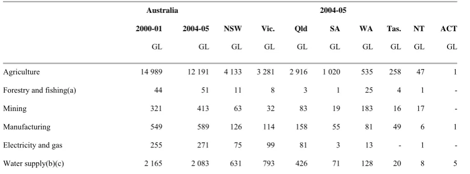
ABS (2006) provides estimates of the quantity of water consumption by state and broad sector, as shown in table 1.
Table 1. Water consumption, 2000-01 and 2004-05
Australia 2004-05
2000-01 2004-05 NSW Vic. Qld SA WA Tas. NT ACT
GL GL GL GL GL GL GL GL GL GL
Agriculture 14 989 12 191 4 133 3 281 2 916 1 020 535 258 47 1
Forestry and fishing(a) 44 51 11 8 3 1 25 4 1
-Mining 321 413 63 32 83 19 183 16 17
-Manufacturing 549 589 126 114 158 55 81 49 6 1
Electricity and gas 255 271 75 99 81 3 13 - 1
Other industries 1 102 1 059 310 262 201 52 168 18 30 17
Household 2 278 2 108 572 405 493 144 362 69 31 31
Total 21 703 18 767 5 922 4 993 4 361 1 365 1 495 434 141 56
- nil or rounded to zero (including null cells)
(a) Includes Services to agriculture; hunting and trapping.
(b) Includes Sewerage and drainage services.
(c) Includes water losses.
Source: ABS (2006) table 1.6.
The following discussion taken from ABS (2006) clarifies exactly what is presented in table 1.
Calculating water use by industries is not straightforward. Water use can include self-extracted water, distributed water, or reuse water, and sometimes a combination of all three sources are used. Calculating water use estimates for an industry or business is made more complicated when water is also supplied to other users, or when water is used in-stream. As such, simply adding self-extracted water, distributed water, and reuse water to derive a figure for total water use can be misleading.
In the Water Account, volumes of water used and supplied by each industry have been balanced to derive 'water consumption'. This figure takes into account the different characteristics of water supply and use of industries and is a way of standardising water use, allowing for comparisons between industries. As such, the following accounting identities have been used:
¾ Total water use is equal to the sum of Distributed water use, Self-extracted water use and Reuse water use;
¾ Water consumption is equal to the sum of Distributed water use, Self-extracted water use and Reuse water use less Water supplied to other users less In-stream use and less Distributed water use by the environment.
For most industries, water use and water consumption are the same as most industries do not have any in-stream use or supply water to other users. However water consumption will be considerably different for some industries, specifically the water supply, sewerage and drainage services industry, electricity and gas supply industry, mining industry, and manufacturing industry where in-stream water use and water supply volumes are significant.
Water consumption rather than water use has been incorporated into MMRF. Water consumption for the ABS broad industry sectors has been split across the more detailed MMRF industries and allocated to intermediate use in proportion to the basic value of the commodity
"WaterSupply". ABS data for household water consumption has been associated with private
consumption of the commodity "WaterSupply".
3. Constructing a baseline for water consumption
The NIAM baseline used in this paper is identical to that used for the CPRS analysis (Centre of Policy Studies (2008)) up to 2008.1 From 2008 onwards projections of future water consumption by users (industries and the residential sector) and states, up to 2023 for industries and 2026 for the residential sector, are incorporated. The compilation of these projections and the information sources used are discussed in subsection 3.1. Beyond the initial period, technical efficiency and consumer preference shifts for water, determined endogenously by the model for the initial period, are continued over the latter period of the baseline but at a decaying rate. The model enhancements required for this projection of past trends at decaying rates are described in subsection 3.2.
A distinctive implementation feature of the NIAM baseline is that it is generated by the RunDynam software as a policy simulation. The new projections of water consumption are
introduced as policy shocks applied to the CPRS baseline. The new 'Make Policy Base' feature of RunDynam then easily allows this policy simulation to be redesignated as the (NIAM) baseline. This process is described in subsection 3.3.
3.1 Projections of water consumption
Two sources were used for the projections of water consumption incorporated in the early years of the baseline: the TERM-H2O baseline underlying the simulations in Dixon et al (2010) and projection of capital city urban water demand in Water Services Association of Australia (2010).
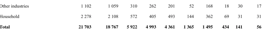
The use of the latter data source is the easiest to describe. It is used to provide an annual growth rate of residential water consumption, from 2009 to 2026, for each state. In the WSAA report, projected demand for water in 2026 is reported, under different population growth assumptions, for all capital cities except Hobart and Darwin. The capital-city average annual growth rate from 2009-2026, for the medium population growth scenario, is used as the growth rate of residential water consumption, from 2009 to 2026, for the associated state/territory. Then, applying these growth rates to MMRF data on water consumption, a growth rate for total residential water consumption across all states and territories, except Tasmania and the Northern Territory, is calculated. This growth rate (which is consequently a weighted average of the rates reported in the WSAA report) is used as the growth rate of residential water consumption, from 2009 to 2026, for Tasmania and the Northern Territory. The residential water consumption growth rates used in the NIAM baseline are shown in table 2.
Table 2. NIAM baseline residential water consumption growth rate from 2009 to 2026
NSW 1.32 VIC 2.08 QLD 4.80 SA 1.37 WA 0.77 TAS 2.45 NT 2.45 ACT 2.04 Total 2.65
Source: Water Services Association of Australia (2010) and MMRF data
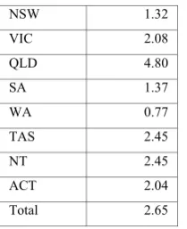
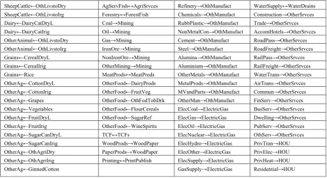
The TERM-H2O baseline is used to provide growth rates in water consumption for each industry from 2008 to 2023 (and for residential consumption from 2008 to 2009) in each state. The mismatch in regional and sectoral coverage between TERM-H2O and MMRF makes this process far from straightforward. Neither the regional nor industry coverage of either model is neatly "nested within" the coverage of the other model. The regional and industry coverage of the two models, and mappings between these dimensions of the two models, are shown in tables 3 and 4, respectively.
Table 3. Mapping between MMRF and TERM-H2O regions
NSW←UpDrlLachNSW NSW←WagCntMrmNSW
NSW←LMrmbNSW NSW←AlbUpMrryNSW
NSW←CentMrryNSW NSW←MrryDrlngNSW
NSW←RofNSW VIC←RoVIC
VIC←MldWMaleeVic VIC←EMalleeVic
VIC←BndNthLodVic VIC←SthLoddonVic
VIC←ShepNGoulVic VIC←SSWGlbrnVic
VIC←OvnsMurryVic QLD↔QLD
SA←RoSA SA←MurrayLndsSA
WA→RoA TAS→RoA
← means many TERM-H2O regions map to MMRF industry
→ means many MMRF regions map to TERM-H2O industry
↔ means one-to-one mapping between an MMRF and TERM-H2O region
The regional mapping is precise, in the sense that there is no region in TERM-H2O that is not the sum of regions in MMRF, or vice versa. The industry mapping is "rougher", as illustrated by the MMRF industries AgServFish and Forestry and the TERM-H2O industries AgriSrvces and ForestFish.
Table 4. Mapping between MMRF and TERM-H2O industries
SheepCattle←OthLivstoDry AgServFish↔AgriSrvces Refinery→OthManufact WaterSupply↔WaterDrains SheepCattle←OthLivstoIrg Forestry↔ForestFish Chemicals→OthManufact Construction→OtherSrvces Dairy←DairyCatDryL Coal→Mining RubbPlastic→OthManufact Trade→OtherSrvces Dairy←DairyCatIrig Oil→Mining NonMetalCon→OthManufact AccomHotels→OtherSrvces OtherAnimal←OthLivstoDry Gas→Mining Cement→OthManufact RoadPass→OtherSrvces OtherAnimal←OthLivstoIrg IronOre→Mining Steel→OthManufact RoadFreight→OtherSrvces Grains←CerealDryL NonIronOre→Mining Alumina→OthManufact RailPass→OtherSrvces Grains←CerealIrig OtherMining→Mining Aluminium→OthManufact RailFreight→OtherSrvces Grains←Rice MeatProds↔MeatProds OtherMetals→OthManufact WaterTrans→OtherSrvces OtherAg←CottonDryL OtherFood←DairyProds MetalProds→OthManufact AirTrans→OtherSrvces OtherAg←CottonIrig OtherFood←FruitVeg MVandParts→OthManufact Commun→OtherSrvces OtherAg←Grapes OtherFood←OthFodTobDrk OtherMan→OthManufact FinServ→OtherSrvces OtherAg←Vegetables OtherFood←FlourCereals ElecCoal→ElectricGas BusServ→OtherSrvces OtherAg←FruitDryL OtherFood←SugarRef ElecGas→ElectricGas Dwelling→OtherSrvces OtherAg←FruitIrig OtherFood←WineSpirits ElecOil→ElectricGas PubServ→OtherSrvces OtherAg←SugarCanDryL TCF↔TCFs ElecNuclear→ElectricGas OthServ→OtherSrvces OtherAg←SugarCanIrig WoodProds→WoodPaper ElecHydro→ElectricGas PrivTran→HOU OtherAg←OthAgriDry PaperProds→WoodPaper ElecOther→ElectricGas PrivElec→HOU OtherAg←OthAgriIrig Printing↔PrintPublish ElecSupply→ElectricGas PrivHeat→HOU OtherAg←GinnedCotton GasSupply→ElectricGas Residential→HOU
← means many TERM-H2O industries map to MMRF industry
→ means many MMRF industries map to TERM-H2O industry
↔ means one-to-one mapping between an MMRF and TERM-H2O industry
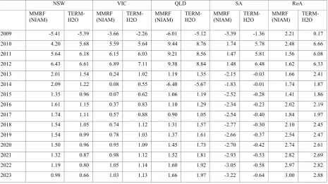
Table 5. Comparison of baseline growth rates of total industry water consumption for MMRF (NIAM) and TERM-H2O
NSW VIC QLD SA RoA
MMRF (NIAM) TERM-H2O MMRF (NIAM) TERM-H2O MMRF (NIAM) TERM-H2O MMRF (NIAM) TERM-H2O MMRF (NIAM) TERM-H2O
2009 -5.41 -5.39 -3.66 -2.26 -6.01 -5.12 -3.39 -1.36 2.21 0.17
2010 4.20 5.68 5.59 5.64 9.44 8.76 1.74 5.78 2.48 6.66
2011 5.64 6.18 6.15 6.03 9.21 8.56 1.47 5.81 1.56 6.08
2012 6.43 6.61 6.89 7.11 9.38 8.84 1.48 6.48 1.62 6.33
2013 2.01 1.54 0.24 1.02 1.19 1.35 -2.15 -0.03 1.66 2.41
2014 2.09 1.22 0.08 0.55 -6.40 -5.67 -1.83 -0.01 1.74 1.87
2015 1.35 0.96 0.07 0.62 1.06 1.19 -2.52 -0.28 1.41 1.86
2016 1.61 1.15 0.37 0.83 1.10 1.29 -2.34 -0.23 2.02 2.19
2017 1.74 1.11 0.57 0.88 0.90 1.05 -2.54 -0.40 1.84 1.97
2018 1.54 1.05 0.74 1.12 1.31 1.57 -2.77 -0.30 2.10 2.45
2019 1.54 0.99 0.78 1.03 1.37 1.61 -2.66 -0.37 2.54 2.47
2020 1.50 0.96 0.95 1.09 1.45 1.73 -2.70 -0.42 2.74 2.61
2021 1.32 0.87 0.98 1.12 1.52 1.81 -2.93 -0.53 2.82 2.69
2022 1.19 0.80 1.05 1.14 1.60 1.92 -3.05 -0.58 2.97 2.82
2023 0.98 0.66 1.03 1.13 1.66 1.97 -3.22 -0.64 3.00 2.88
Source: TERM-H2O baseline used in Dixon et al (2010); ABS (2006); MMRF baseline used in Centre of Policy Studies (2008).
Most noteworthy in table 5 are the differences between baseline growth rates for South Australia (and to a lesser extent the rest of Australia state aggregate). Plainly the differing industry aggregations of the two models will lead to some differences in the growth rates. But it seems that the source of discrepancies may be more related to different sources of water consumption data. Indeed, table 6 highlights the differences in the 2008 shares of total water consumption data by broad sectors for the two models.
Table 6. Comparison of 2008 water consumption shares by broad sector for MMRF (NIAM) and TERM-H2O
NSW VIC QLD SA RoA
MMRF
(NIAM) TERM-H2O MMRF (NIAM) TERM-H2O MMRF (NIAM) TERM-H2O MMRF (NIAM) TERM-H2O MMRF (NIAM) TERM-H2O
AgrForFsh 0.69 0.67 0.65 0.52 0.66 0.58 0.74 0.61 0.38 0.25
Min 0.01 0.01 0.01 0.01 0.02 0.02 0.02 0.02 0.12 0.14
Manu 0.02 0.02 0.02 0.03 0.04 0.05 0.04 0.07 0.06 0.08
Serv 0.18 0.19 0.24 0.32 0.17 0.21 0.10 0.14 0.20 0.24
Residential 0.10 0.11 0.09 0.11 0.12 0.14 0.11 0.16 0.24 0.29
Some reconciliation of data sources ABS (2006) and ABS (2008) and/or how they have been allocated across activities in the model databases would be helpful.
3.2 Continuation of past trends in water consumption
In the NIAM baseline water consumption by industries and the residential sector is imposed exogenously, up to 2023 for industries and 2026 for the residential sector. To achieve this the model variable xwater, the percentage growth rate of water consumption dimensioned across all
users (industries and the residential sector) and states and territories, is made exogenous and shocked with the projected growth rates of water consumption. The instruments used to accommodate these shocks are the components of technical efficiency variable acomind and
consumer preference variable a3tot corresponding to the commodity "WaterSupply".
A decision must be made as to how trends in water consumption are extrapolated beyond the years for which projections of water consumption have been incorporated in the baseline.
One possibility is to have no further technical efficiency or preference changes for water beyond the period for which projections have been formulated. This seems unsatisfactory as it disregards what the model has determined is the recent trends in these variables necessary to accommodate the projections.
A second possibility is to continue the growth rates in technical efficiency and preferences at the values determined in the final years for which projections were imposed on the model. This approach has the virtue of taking what is implied by the model seriously, but runs the risk of overestimating what is possible in the future by an extrapolation of a past trend at the same intensity. For example, the TERM-H2O baseline implies large declines in water consumption by certain agricultural sectors. Even though it is not the trends in actual water consumption but the model inferred technical efficiency trends that would be continued into the future, to continue these efficiency trends unabated may lead to unrealistically low water consumptions.
A third possibility is intermediate between these two: to continue the growth rates in technical efficiency and preferences multiplied by a decay factor. This is the approach that was taken in the NIAM baseline. Some new equations were introduced to MMRF to facilitate this. In fact, the new equations are capable of facilitating any of the three possibilities just outlined (by selecting the decay factor to be 0, between 0 and 1 or 1, respectively). An excerpt of the new equations (and associated TABLO code) are shown in figure 1. Note that only the code pertaining to the industry technical efficiency variable acomind is shown. In the model there is
corresponding code for the consumer preference variable a3tot.
The idea underlying this code is as follows. Let:
=
t
a percent change in technical efficiency in year t;
t
t a
A = 1+ the index of technical efficiency change in year t; and
=
(
1)
1 1 1 1 1 − ⋅ + = ⋅ + = + = + + t t t t A a a A δδ (E1)
In the TABLO code, the first expression in brackets on the right-hand-side of Formula & Equation E_d_acomind, is equation (E1) with all terms moved to the left-hand-side:
r) i, c, ACOMIND_L( 1 ⇔ + t A r) i, B(c, ACOMIND_L_ ⇔ t A r) i, c, DCYCOMIND( ⇔ δ
Levels variable ACOMIND_L is initially set equal to 1. During the solution procedure for a
particular year the levels variable Unity (which is associated with the MMRF momentum variable d_unity) changes from 0 to 1. If levels variable D_ACOMIND_L is exogenous and shocked to a
final value of zero then equation (E1) is satisfied by the end of the solution procedure.
The decay factor has been declared as a levels variable with all components set to an initial value of 1 or conditionally read from the file MDATA. The decay factor has also been given the
full dimension of the technical efficiency variable. This allows the model user maximum flexibility in setting the values of the decay factor - it can vary across industries, commodities and regions and across time. The default decay factor of 1 (the value assigned to the decay factor if the model user neither specifies values on the file MDATA nor assigns values by shocking the
levels variable DCYCOMIND) causes past growth in technical efficiency to be continued into the
future.
A decay factor of δ =0.5 was used in the current study.
Note that the commodity dimension of the TABLO code in figure 1 is COM1, a
user-specified subset of the full set of commodities COM. For the current exercise COM1 has just one
Figure 1. TABLO code for implementing continuation of past technical efficiency trends at a decaying rate
3.3 Implementation details of NIAM baseline - use of RunDynam
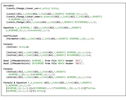
As mentioned at the beginning of section 3, the NIAM baseline is substantially the same as the CPRS baseline (Centre of Policy Studies (2008)) but with amended projections of water consumption. A decision was made to implement these changes to water consumption as a policy simulation relative to the CPRS baseline. The policy closure in this context is very similar to the forecasting closure. Only a few swaps are required to impose water consumption projections exogenously or continue forward in time (at a decaying rate) model determined growth in technical efficiency and consumer preferences. The closure swaps are shown in figure 2.
Variable
(Levels,Change,Linear_var=d_unity) Unity;
(Levels)(All,c,Com1)(All,i,Ind)(All,r,REGDST) ACOMIND_L(c,i,r);
(Levels,Change,Linear_name=d_acomind)(All,c,Com1)(All,i,Ind)(All,r,REGDST) D_ACOMIND_L(c,i,r);
(Levels,Change)(All,c,Com1)(All,i,Ind)(All,r,REGDST) DCYCOMIND(c,i,r);
Equation E_p_ACOMIND_L (All,c,Com1)(All,i,Ind)(All,r,REGDST) p_ACOMIND_L(c,i,r)=acomind(c,i,r);
Coefficient
(Parameter)(All,c,Com1)(All,i,Ind)(All,r,REGDST) ACOMIND_L_B(c,i,r);
Formula
(Initial) Unity=0;
(Initial)(All,c,Com1)(All,i,Ind)(All,r,REGDST) ACOMIND_L(c,i,r)=1; (Initial)(All,c,Com1)(All,i,Ind)(All,r,REGDST) DCYCOMIND(c,i,r)=1;
Read (IfHeaderExists) ACOMIND_L from file MDATA header "ACI";
Read (IfHeaderExists) DCYCOMIND from file MDATA header "DKCI";
Formula
(Initial)(All,c,Com1)(All,i,Ind)(All,r,REGDST) ACOMIND_L_B(c,i,r)=ACOMIND_L(c,i,r);
(Initial)(All,c,Com1)(All,i,Ind)(All,r,REGDST) ACOMIND_L(c,i,r)=1;
Formula & Equation E_d_acomind (All,c,Com1)(All,i,Ind)(All,r,REGDST) D_ACOMIND_L(c,i,r)=
Figure 2. Closure swaps for incorporating water consumption projections
The strategy of adding a limited amount of new information to an already sound baseline via a policy simulation is an approach that allows baseline development to take place in small increments. Once the new information has been satisfactorily incorporated into the baseline, the RunDynam option 'Make Policy Base' can be used to rename files, reset options and produce new closure and shock files so that the RunDynam policy simulation (which is the NIAM baseline in the current application) becomes the RunDynam baseline.
4. Disaggregation of the water supply industry
The proof-of-concept simulation undertaken in this paper is reduced water availability. This simulation was chosen in consideration of the possible impacts of climate change on water availability. However, not all water supply options are equally dependent on climate and rainfall. Indeed, in recent years desalination technology has been introduced in many states as an insurance policy against extreme drought conditions and the possible longer term impacts of climate change both on total rainfall and the variability of rainfall.2
In the version of MMRF used for the analysis of the CPRS, there is only one water supply industry. This is not much of a limitation when MMRF is being used to examine the impacts on the economy of reducing greenhouse gas emissions. But for examining the impacts of climate change on the economy, and particularly for the proof-of-concept simulation undertaken in this paper, a range of water supply options need to be considered to realistically represent the economic impacts.
2 The term "insurance policy" is used quite deliberately. It anticipates the difficult issue of the appropriate discount rate to use for calculating a rental to capital from the construction cost of desalination supply options.
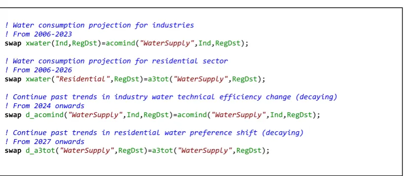
! Water consumption projection for industries ! From 2006‐2023
swap xwater(Ind,RegDst)=acomind("WaterSupply",Ind,RegDst);
! Water consumption projection for residential sector ! From 2006‐2026
swap xwater("Residential",RegDst)=a3tot("WaterSupply",RegDst);
! Continue past trends in industry water technical efficiency change (decaying) ! From 2024 onwards
swap d_acomind("WaterSupply",Ind,RegDst)=acomind("WaterSupply",Ind,RegDst);
! Continue past trends in residential water preference shift (decaying) ! From 2027 onwards
The analysis of the CPRS necessitated the introduction of a technology bundle (Hinchy and Hanslow (1996)) for electricity production. The different carbon-intensities of the available and potential technologies means that significant substitution between technologies will occur in response to a sufficiently high price on carbon. Similarly, in the present context, a technology bundle needs to be introduced for water supply, to capture the different climate-sensitivities of various supply options.
The water supply industry was disaggregated into three industries, which all supply the one commodity "WaterSupply". The three industries were Surface & Groundwater (which
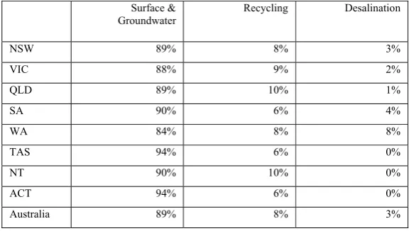
encompasses the most climate-sensitive supply option based on rainfall and dam levels), recycling and desalination. The water accounts in ABS (2006) provide data on water supply by these three options by state, but recycling and desalination have grown rapidly since then. To obtain estimates of current output shares for these supply options the following procedure was used. Once the water accounts have been incorporated in MMRF, the MMRF baseline provides estimates of water consumption in 2009 Various water authorities (Our Water Our Future(2010), SA Water (2010), WaterSecure (2010), WA Water Corporation (2010a), WA Water Corporation (2010b)) provide information on the output of desalination plants in, or close to, the year 2010. Table 1.18 of ABS (2006) provides estimates of use of reuse water supplied by urban water authorities in 2004-05 for each state. We use these quantities of water use as a share of total water consumption as estimates of the share of recycled water for each state in 2004-05. Sydney Water (2009) provides information on total demand and recycling in the greater Sydney region. This share of recycling is assumed to be representative of NSW as a whole for 2009. The growth in this share relative to the NSW share inferred from ABS (2006) is assumed to apply to other states also, thus providing estimates of the 2009 share of recycled water in total water consumption for all states. The estimates of 2009 output shares for the three water supply options are shown in table 7.
Table 7. Share of water supplied by different water supply options (2009)
Surface &
Groundwater Recycling Desalination
NSW 89% 8% 3%
VIC 88% 9% 2%
QLD 89% 10% 1%
SA 90% 6% 4%
WA 84% 8% 8%
TAS 94% 6% 0%
NT 90% 10% 0%
ACT 94% 6% 0%
Australia 89% 8% 3%
The shares in table 7 are used to disaggregate the water supply industry in the MMRF database into three industries with an identical cost structure.3 This is a simple disaggregation that preserves the balance of the database without any need for invoking RAS procedures. If no differential shocks are applied to the three water supply industries, the output shares of the three industries will remain constant at their initial values. This is what is done when generating the NIAM baseline until 2010 when:
¾ the distinctive cost structure of the desalination industry is introduced via an input demand twist; and
¾ the output shares of water supply technologies are held unchanged via technical efficiency changes that are cost-neutral for the three water supply industries as a whole. Thus the model is used to alter the input cost structures of the three water supply industries. This ensures that database balance in maintained. This process, and the data for desalination input costs, are discussed in the section 5.
5. Cost-neutral reconfiguration of a technology bundle - introducing the water desalination technology input cost structure
The incorporation of a water supply technology bundle is important because of the varying degrees of climate dependency of the different water supply options. But, from the point of view of greenhouse emissions and climate change, another important reason for introducing this technology bundle is the differing input requirements of the technologies, in particular, the energy intensity of the desalination technology. For example, in considering the options for a desalination plant to supply drinking water to the greater Sydney region, Sydney Water (2005) contains extensive discussion of the source of electricity for the plant (grid versus on-site gas-fired generator) and the greenhouse emissions. In subsection 5.1 we discuss the input cost data for the desalination technology, and compare it with the input cost structure of the water supply industry as a whole. In subsection 5.2 we describe the model modifications introduced to allow the input cost data for the desalination technology to be incorporated in the model database as part of the NIAM baseline generation. This innovation may be of more general applicability. So subsection 5.3 provides a brief discussion of its potential wider application and limitations.
5.1 Desalination input cost data
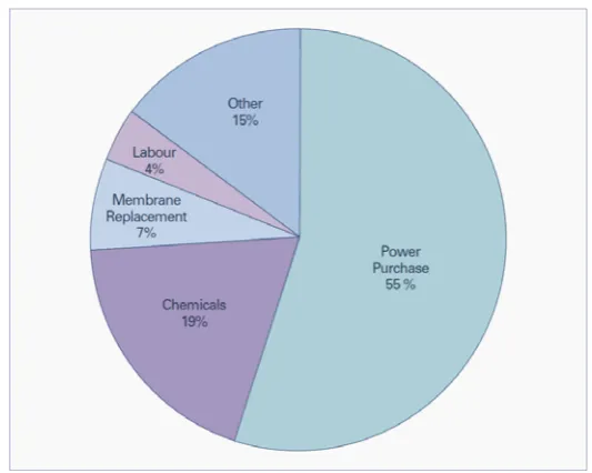
Sydney Water (2005) provides the operating cost breakdown shown in figure 3.
Figure 3. Operating Cost Breakdown for a 500ML/day Desalination Plant
Source: Sydney Water (2005) figure 8.3.
These inputs concord well with commodities in the MMRF database, as shown in table 8.
Table 8. Major inputs to desalination technology
Desalination plant inputs MMRF commodity/primary factor
Chemicals Chemicals Membrane replacement RubbPlastic
Power purchase ElecSupply
Labour Labour
The major cost item missing is the rental cost of capital. This can be calculated using information on the capital cost of a desalination plant, the time to construct the plant and an assumption about the discount rate to be used in annualising the capital cost into a rental. The first two data are contained in Sydney Water (2005) table 8.1, and are $1.75 billion and 26 months, respectively, for a plant of the size that has subsequently been constructed in Sydney. The choice of a discount rate is not straightforward. As alluded to at the beginning of section 4, the construction of a desalination plant is an insurance policy. As stated among the key findings of Sydney Water (2005):
In the event of ongoing severe drought, desalination represents a viable method of supplementing supplies of drinking water for Sydney, despite having a relatively high cost of water compared to current sources of supply.
carting). For calculating rentals to capital in the desalination technology in the current exercise a discount rate of 10 per cent has been used. This implies an annual rental to capital of $177,411,757.
The total operating costs of running a 500 megalitre per day desalination plant at full capacity 94 per cent of the time is $1.44 per kilolitre. (Sydney Water (2005) section 2.2.1). The annual operating cost implied by this ($262.8 million) can be used with the annual capital rental to calculate the share of capital rentals in total costs as:
$177,411,757/($177,411,757+$262,800,000) = 0.40
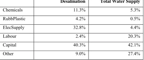
The shares of all inputs in total costs, for the desalination technology and for the water supply industry as a whole (the latter from the MMRF database), are shown in table 9.
Table 9. Input cost shares of desalination technology versus total water supply
Desalination Total Water Supply
Chemicals 11.3% 5.3%
RubbPlastic 4.2% 0.5%
ElecSupply 32.8% 4.4%
Labour 2.4% 20.3%
Capital 40.3% 42.1%
Other 9.0% 27.4%
Source: Sydney Water (2005); MMRF database.
There is a significant difference in the input cost shares that is of particular relevance in the context of greenhouse gas emissions, desalination being a much more electricity intensive supply option.
For this early stage of NIAM development it is assumed that the input cost structures of the two non-desalination water-supply technologies - Surface & Groundwater and recycling - are identical.
5.2 Cost-neutral imposition of new input costs
In the MMRF model, a twist is a set of changes in the technical efficiency of industry inputs that does not contribute to a change in total industry costs. An example of a twist is the import/domestic twist, which can be used to make an industry more or less intensive in the use of the imported variants of commodities. Another example is the labour-capital twist.
To enable the cost structure of the desalination technology to be introduced into the NIAM baseline, a twist that applies to all industry inputs is introduced. The name of the twist variable is
twist1inp. It is dimensioned over all industry inputs - commodities; the primary factors of labour,
capital and land; other costs; and purchases from the national electricity market (NEM). As shown in Equation E_twist1inp of figure 4, twist1inp is expressed as the sum of two component
variables - ftwist1inp, which is the instrument for targetting a particular industry input, and twist1,
input-cost share (levels variable S1INP) weighted sum of twist1inp, across all inputs for each industry,
is zero. This is implemented in Equation E_twist1 of figure 4. Note that although twist1inp ranges
across all industries, its component variables - ftwist1inp and twist1 - are restricted to only range
across the industries for which the twists are to be used - the three water supply industries (specified in the new set WaterSupply introduced as part of the disaggregation).4 To introduce the
all input twist mechanism into each industry's input demand equations, the variable twist1inp is
added to the demand equations. For example, for commodity demands by industries the equation becomes:
Equation E_x1o # Demands for composite inputs, User 1 #
(all,c,COM)(all,i,IND)(all,q,REGDST)
x1o(c,i,q) = x1tot(i,q) + acomind(c,i,q) + IF{V1PURO(c,i,q)>0, a1(i,q) + a1o(c,i,q) + acom(c,q) + natacom(c) + agreen(c,i,q) +
elecsub(c,i,q) + transub(c,i,q) + meatsub(c,i,q) +
heatsub(c,i,q) + processsub(c,i,q) + twist1inp(c,i,q)};
In year 2010 of the NIAM baseline generation the all input twist mechanism is invoked by the closure swaps and shocks shown in figure 5. Input shares for each technology, for all of the major inputs to the desalination technology, are set by the TFinal_level statement.5 The
corresponding components of the variable ftwist1inp adjust the input demands to conform with
these shares. The cost-neutralising variable twist1 adjusts all non-major inputs to ensure that the
input cost share S1INP sums to one across all inputs for each of the water supply technologies.
A twist is cost-neutral in the sense that a shock to a twist variable does not itself contribute to a change in costs.6 But a twist will affect the inputs used by an industry, and as these inputs may have different price changes, the presence of a twist may lead to different industry costs than would otherwise be the case. Consequently, the twist used to introduce the desalination technology input structure will, on its own, lead to an alteration in the output shares of the water supply technologies. But we would want to keep these constant at the shares used to disaggregate the database, which pertained to 2009 (as close as we could get to the current year 2010).
4 The MMRF used for the CPRS had one WaterSupply industry producing a commodity called WaterSupply. For NIAM, MMRF has been disaggregated to incorporate a water supply technology bundle that has a set of three industries called, collectively, WaterSupply. Each of these three industries produces the same commodity called WaterSupply. Confused yet!
5 The input cost shares for the non-desalination technologies are, for this stage of NIAM development, assumed to be identical.
Figure 4. TABLO code to allow twists across all industry inputs
Figure 5. Closure swaps and shocks to implement all input twist mechanism
for water supply technologies
So we introduce what is effectively another twist mechanism to preserve the output shares of the water supply technologies. The TABLO code to implement this is shown in figure 6, while the closure swaps are shown in figure 7.
Set Ind1=WaterSupply;
Variable
(All,i,Inputs)(All,j,Ind1)(All,r,RegDst) ftwist1inp(i,j,r) #Exogenous component of twist on all industry inputs#; (All,j,Ind1)(All,r,RegDst) twist1(j,r)
#Cost‐neutralising offset for twist on all industry inputs#;
(Levels)(All,i,Inputs)(All,j,Ind1)(All,r,RegDst) S1INP(i,j,r) #Share of inputs in total costs#;
Formula
(Initial)(All,i,Inputs)(All,j,Ind1)(All,r,RegDst) S1INP(i,j,r)= {sum[k,Com:k=i,V1PURO(k,j,r)]+IF[i="lab",V1LAB_O(j,r)]+ IF[i="cap",V1CAP(j,r)]+IF[i="lnd",V1LND(j,r)]+
IF[i="oct",V1OCT(j,r)]+IF[i="nem",ISSUPPLY(j)*V1NEM(r)]}/id01[COSTS(j,r)];
Equation E_p_S1INP (All,i,Inputs)(All,j,Ind1)(All,r,RegDst) p_S1INP(i,j,r)=
{sum[k,Com:k=i,p1o(k,j,r)+x1o(k,j,r)]+ IF[i="lab",p1lab_o(j,r)+x1lab_o(j,r)]+
IF[i="cap",p1cap(j,r)+x1cap(j,r)]+IF[i="lnd",p1lnd(j,r)+x1lnd(j,r)]+ IF[i="oct",p1oct(j,r)+x1oct(j,r)]+
IF[i="nem",ISSUPPLY(j)*(p8tot+x1NEM(r))]}‐{p1tot(j,r)+x1tot(j,r)};
Equation E_twist1inp (All,i,Inputs)(All,j,Ind)(All,r,RegDst) twist1inp(i,j,r)=sum[k,Ind1:k=j,ftwist1inp(i,k,r)+twist1(k,r)];
Equation E_twist1 (All,j,Ind1)(All,r,RegDst)
0=sum{i,Inputs,S1INP(i,j,r)*[ftwist1inp(i,j,r)+twist1(j,r)]};
XSet DesalInp (Chemicals, RubbPlastic,
ElecSupply, Lab, Cap);
XSubset DesalInp is subset of Inputs;
swap
p_S1INP(DesalInp,WaterSupply,RegDst)=ftwist1inp(DesalInp,WaterSupply,RegDst);
Figure 6. TABLO code to preserve output shares of water supply technologies
Figure 7. Closure swaps to preserve output shares of water supply technologies
In the TABLO code of figure 6 three new variables are defined. The levels variable
S0WATSUP is the share of each water supply technology in total water supply. The variable x0watsup is the percentage change in the total quantity of water supplied. The variable a0watsup
is the percentage change in the total technical efficiency of all three water supply technologies. To understand how these variables are used in the closure swaps of figure 7, it helps to review how the NIAM baseline is being generated.
The NIAM baseline is generated in RunDynam as a policy simulation with respect to the CPRS baseline. When the CPRS baseline was originally produced in Centre of Policy Studies (2008), it contained only a single water supply industry. Once the water supply industry is disaggregated into three technologies the CPRS baseline is rerun but with no shocks introducing the distinctive cost structure of the desalination technology. Thus all three water supply technologies grow at the same rate and, consequently, in all years of the CPRS baseline maintain the same (2009) output shares in table 7. The CPRS baseline has a cost-neutralising mechanism that can be applied across many of the industry technical efficiency variables. The equation driving this mechanism is invoked by making the variable d_fa1 exogenous and the general
industry productivity variable a1 endogenous. In the policy simulation generating the NIAM
baseline, the first closure swap of figure 7 has the effect of releasing the cost-neutralisation Variable
(Levels)(All,i,WaterSupply)(All,r,RegDst) S0WATSUP(i,r); (All,r,RegDst) x0watsup(r) #Water supply by state#; (All,r,RegDst) a0watsup(r)
#Overall technical efficiency of water supply by state#;
Formula
(Initial)(All,i,WaterSupply)(All,r,RegDst) S0WATSUP(i,r)= MAKE("WaterSupply",i,r)/id01[MAKE_I("WaterSupply",r)];
Equation E_p_S0WATSUP (All,i,WaterSupply)(All,r,RegDst) p_S0WATSUP(i,r)=x1tot(i,r)‐x0watsup(r);
Equation E_x0watsup (All,r,RegDst)
x0watsup(r)=sum[i,WaterSupply,S0WATSUP(i,r)*x1tot(i,r)];
Equation E_a0watsup (All,r,RegDst)
id01{sum[i,WaterSupply,COSTS(i,r)]}*a0watsup(r)= sum[i,WaterSupply,COSTS(i,r)*a(i,r)];
swap p_S0WATSUP=d_fa1(WaterSupply,RegDst);
mechanism and allowing the variable a1 to adjust so that the output shares S0WATSUP are
maintained at the CPRS baseline level (which equals the target levels from table 7). Now, of course, the set of output shares are not independent. Given values for any two shares the third is determined so that all shares sum to one. So the first swap of figure 7 alone would lead to a singularity. The second swap of figure 7 endogenises one of the output shares (it does not matter which one) and exogenises the variable a0watsup, that is, the total technical efficiency of all
water supply. Thus a0watsup is set at the same value as determined in the CPRS baseline. This is
again another example of a cost-neutralising mechanism, this time across a set of industries (the three water supply technologies). In the NIAM baseline, for the year 2010, the technical efficiency of each of the three technologies is different to the CPRS baseline, but for water supply as a whole the technical efficiency is the same.
5.3 Applicability and limitations of cost-neutral imposition of new input costs
Caution is required in translating a twist in a baseline into technical efficiency shocks to be applied in the policy simulation. It is not (usually) correct to merely keep the value of the twist variable the same in both. Because shares are different in the baseline and policy simulation, the sets of technical efficiency shocks that are equivalent to a given value of the twist variable differ between the two. Consequently, to apply the same value to the twist variable in both the baseline and policy simulation will introduce different regimes of technical efficiency changes and lead to spurious extra output losses or gains in the policy simulation relative to the baseline.
Such potential problems with the all input twist mechanism are avoided in the current application because the proof-of-concept policy simulation (of reduced water availability) commences in year 2011. The NIAM baseline leading up to 2010, and in particular the all input twist mechanism, really just serves to produce the database from which the proof-of-concept policy simulation commences.
In the current application the inclusion of a water supply technology bundle has been implemented by:
¾ an initial disaggregation of the water supply industry into three industries with identical technology but different levels of output; and
¾ subsequent use of the model and the all input twist mechanism to invoke the distinctive cost structure of new industries.
These two steps have been used merely as a data generation process. An alternative approach is to use the model to undertake an historical simulation that reproduces the growth in the new technologies from 2005-2010 using as instruments those model variables that best represent what has changed in reality to induce the observed growth in new technologies. The steps for undertaking such an historical simulation approach would be:
¾ an initial disaggregation of the water supply industry into three industries with different technologies and different levels of output (perhaps very low for the desalination technology for some states);
¾ probable rebalancing of the database with a RAS;
¾ identifying the variables to be used as instruments (perhaps the shifter variable f_eeqror
¾ by a closure swap of instruments and targets, solve the model from 2005-2010 to determine the values of the instruments that induce the observed growth in technologies; and
¾ assess the reasonableness and realism of the instrument values found.
Clearly the historical simulation approach is complicated. It has the advantage of possibly providing insights into economic change over the historical period that could inform the construction of the baseline in future years. But it is a challenging exercise which, in this application, confronts the issue of growing a new industry (desalination) from a low base. So for this early proof-of-concept stage of NIAM development a simpler procedure for introducing the water supply technology bundle has been used.
6. Reduced water availability - impacts of climate change and formulating the model shocks
The proof-of-concept simulation is holding the quantity of water supplied from sources other than recycling and desalination fixed at 2010 levels in each state. This is a simple and adequate way of assessing the value of model development to date, gaining some important insights into the effects of reduced water availability and identifying shortcomings in the current model structure and database.
Plainly it would be valuable to adjust the simulation to more adequately represent the changes in water availability suggested by climate change research, and how these changes may vary between regions. CSIRO research inputs, such as CSIRO (2010), will be critical in this regard.
7. Proof of concept simulation results - reduced water availability
This section discusses the proof-of-concept simulation setup and results. Subsection 7.1 describes the closure and shock files used to run the proof-of-concept simulation as a policy simulation with the RunDynam software. Subsections 7.2 and 7.3 examine the national level macroeconomic and sectoral results, respectively. Of particular interest is substitution within the water-supply technology bundle, the most significant new feature added to the model, and its implications for the structure of the economy. Subsection 7.4 looks at state macro results and how and why they differ between states.
7.1 Model closure and shocks
Labour markets
employment is determined by demographic factors, which are largely unaffected by reduced water availability.
At the regional level, labour is assumed to be mobile between state economies. Labour is assumed to move between regions so as to maintain inter-state wage differentials at their levels in the baseline. Accordingly, regions that are relatively favourably affected by reduced water availability will experience relative increases in employment at the expense of regions that are relatively less favourably affected.
MMRF lacks the necessary demographic detail to allow for a full explanation of changes in population and labour supply in response to reduced water availability. Accordingly, in the policy simulations, population and participation rates are exogenously set at baseline levels.
Private consumption and investment
Consumption expenditure of the regional household is determined by Household Disposable Income (HDI). HDI is the sum of payments to domestic labour and capital and government transfer payments net of direct taxation.
Investment in all but a few industries is allowed to deviate from its value in the baseline in line with deviations in the expected rate of return on the industry's capital stock. Investors are assumed to base their decisions on the current state of the economy, that is, expected rates of return are assumed to move with contemporaneously observed rates of return.
Rates of return on capital
Under the policy scenarios, MMRF allows for short-run divergences in rates of return on industry capital stocks from their levels in the baseline. Such divergences cause divergences in investment and hence capital stocks. The divergences in capital stocks gradually erode the divergences in rates of return, so that in the long-run rates of return on capital over all regional industries return to their baseline levels.
Government budget balances
The budget balances as a share of nominal GDP of all governments, state and Federal, are fixed at their values in the reference case. Budget balances are constrained via endogenous movements in lump-sum payments to households.
Production technologies and household tastes
MMRF contains many types of technical change variables. In the policy simulation it is assumed that all technology variables have the same values as in the baseline.
Land for agriculture and forestry
agricultural and forestry use is fixed Thus, if the demand for land in the more water-intensive agricultural industries decreases, land will shift to other agricultural uses or to forestry.
The numeraire price
While MMRF determines all relative prices endogenously, one nominal price variable in the model must be exogenous. This variable will, unless shocked in the policy simulation, be unchanged from the baseline. The consumer price index (CPI) has been made exogenous in the proof-of-concept policy simulation. This means that in the policy simulation the nominal exchange rate adjusts from one year to the next to ensure that the inflation rate is the same as in the baseline. As there is not monetary sector in MMRF, the model does not provide any indication of what adjustments in monetary variables occur.
Imposition of reduced water availability
For each state, from the year 2011 onwards, the output of water from the "Surface & Groundwater" water-supply technology is held fixed at 2010 levels. This is achieved by making the output of this technology exogenous and the shifter on the price of other cost tickets exogenous, as follows:
Figure 8. Closure swaps and shocks for reduced water availability
This closure swap and shock statement are applied from year 2011 onwards of the proof-of-concept policy simulation. Note that a target shock (tshock) statement is used to ensure that, in
the policy simulation, there is zero growth in the targetted components of variable x1tot
regardless of the baseline growth rate in the corresponding year. Consequently the severity of the shock will depend on what has been assumed about water availability in the baseline. This is governed largely by the projections of water demand incorporated in the baseline (subsection 3.1). The effect of the closure swap and shock from figure 8 is to reduced the supply of water, thus leading to an increase in the price of water.7
7 Or at least the shadow price of water. If the price of water is regulated and held at a value below this shadow price, then other regulatory mechanisms (such as restrictions) may need to be introduced. What has been modelled assumes that, whatever regulation is imposed, the effect is equivalent to a price mechanism.
swap f1oct("WatOther",RegDst)=x1tot("WatOther",RegDst);
7.2 National macroeconomic results
Figures 10 to 15 show various national aggregates, arranged so as to illuminate the mechanisms operating in the policy simulation. All results are percent changes relative to the baseline, except where it is indicated in the naming of a variable that it is a change. The shock applied to the model is a supply-side shock that increases in magnitude over time. Its effects differ in the short versus long-run, non only because of the increasing magnitude of the shock, but because of the progressive reallocation of resources within the economy over time.
Short-run (2011-2016)
In the short-run the structure of the economy cannot easily change in response to an increase in the price of water. At this early stage of NIAM development, industries have not been modelled as being able to substitute between water and other intermediate inputs or primary factors. In the short-run capital stocks in each industry and region are fixed. Consequently, given the limited substitution possibilities in the short-run, the economy responds with a decline in the returns to primary factors. As wages are sticky in the short-run, they cannot decline enough to keep employment at its baseline level. Consequently, both employment and wages decline. The reduction in rates of return to capital leads to a decline in investment. The reduction in domestic activity, particular in investment, leads to a reduction in imports. Further, goods no longer demanded in the domestic market are exported, the decline in factor prices offsetting the price increase in water and making Australian goods cheaper on the international market. Consequently, exports increase. The only other component of GDP to increase in the short-run is government consumption. The closure used specifies that nominal government consumption moves in line with nominal GDP. But the government consumption price index is the lowest (in the short to medium term) of all price indices of expenditure components of GDP, because of the distinctive composition of government consumption. Real private consumption, on the other hand, declines, as its price index is the highest for all expenditure components of GDP (figure 12 - recall that the CPI is the numeraire so its graph will be the horizontal axis).
Medium-run (2016-2030)
upwards, eventually rising above baseline. Briefly rates of return are even higher than in the baseline, as can be seen by the rental price of capital rising above the investment price index in figure 13.
The trending up of all primary factor prices from 2023, and the associated increase in investment, leads to an increase in imports and decrease in exports until imports rise above, and exports fall below, their baseline values (in 2028 and 2025, respectively).
Long-run (2030 onwards)
From 2030 onwards real wages are rising so as to bring employment back to its baseline level, which occurs toward the end of the simulation time period. The decline in employment leads to a decline in the marginal product of capital and in investment. The latter falls gradually back to near baseline levels, and so capital gradually converges to a constant deviation from its baseline value.
Figure 9. National macro results -real GDP and components
(deviation from baseline)
‐1.2 ‐1 ‐0.8 ‐0.6 ‐0.4 ‐0.2 0 0.2 0.4 0.6
2011 2012 2013 2014 2015 2016 2017 2018 2019 2020 2021 2022 2023 2024 2025 2026 2027 2028 2029 2030 2031 2032 2033 2034 2035 2036 2037 2038 2039 2040 2041 2042 2043 2044 2045 2046 2047 2048 2049 2050 2051
Real GDP Real private consumption Real investment Real government consumption Real exports Real imports
Figure 10. National primary factor markets
(deviation from baseline)
‐2 ‐1.5 ‐1 ‐0.5 0 0.5 1
2011 2012 2013 2014 2015 2016 2017 2018 2019 2020 2021 2022 2023 2024 2025 2026 2027 2028 2029 2030 2031 2032 2033 2034 2035 2036 2037 2038 2039 2040 2041 2042 2043 2044 2045 2046 2047 2048 2049 2050 2051
Employment Capital stock Nominal price of labour Nominal price of capital Nominal price of land
Figure 11. Price indices of expenditure components of GDP relative to CPI
(deviation from baseline)
‐0.9 ‐0.8 ‐0.7 ‐0.6 ‐0.5 ‐0.4 ‐0.3 ‐0.2 ‐0.1 0
2011 2012 2013 2014 2015 2016 2017 2018 2019 2020 2021 2022 2023 2024 2025 2026 2027 2028 2029 2030 2031 2032 2033 2034 2035 2036 2037 2038 2039 2040 2041 2042 2043 2044 2045 2046 2047 2048 2049 2050 2051
Investment price index Federal government consumption price index
Domestic‐currency export price index, fob Domestic‐currency import price index, cif
GDP price index
Figure 12. Investment behaviour
(deviation from baseline)
‐1.2 ‐1 ‐0.8 ‐0.6 ‐0.4 ‐0.2 0 0.2 0.4 0.6 0.8
2011 2012 2013 2014 2015 2016 2017 2018 2019 2020 2021 2022 2023 2024 2025 2026 2027 2028 2029 2030 2031 2032 2033 2034 2035 2036 2037 2038 2039 2040 2041 2042 2043 2044 2045 2046 2047 2048 2049 2050 2051
Figure 13. National changes in alternative supplies of water
(deviation from baseline)
0 0.05 0.1 0.15 0.2 0.25 0.3 0.35 0.4 0.45 0.5
2011 2012 2013 2014 2015 2016 2017 2018 2019 2020 2021 2022 2023 2024 2025 2026 2027 2028 2029 2030 2031 2032 2033 2034 2035 2036 2037 2038 2039 2040 2041 2042 2043 2044 2045 2046 2047 2048 2049 2050 2051
Change in share of recycling Change in share of desalination
Figure 14. National water supply and price
(deviation from baseline)
‐15 ‐10 ‐5 0 5 10 15
2011 2012 2013 2014 2015 2016 2017 2018 2019 2020 2021 2022 2023 2024 2025 2026 2027 2028 2029 2030 2031 2032 2033 2034 2035 2036 2037 2038 2039 2040 2041 2042 2043 2044 2045 2046 2047 2048 2049 2050 2051
Summary
The decrease in the availability of water induces two types of price response. The first is an increase in the price of water. The second is a decrease in primary factor prices. The magnitudes of these vary over time, both in response to an increasing shock but also to the extent that resources can reallocate between activities in response to the price changes thus tending to reduce the magnitude of the price changes. This is particularly so with regard to substitution toward alternative water supply options, but also at play is the stickiness of real wages and the response of investment to current period rates of return. In the short-run scale effects dominate substitution effects. Resources are less able reallocate and the impact is more a reduction in domestic demand and larger reductions in primary factor prices leading to an increase in exports. The deviation of the price of water above baseline is increasing over time. In the medium to long-run there is less of a scale effect and more of a substitution effect, in the sense of resources moving between activities towards alternative means of water supply and less water intensive production. The lessening of the reduction in domestic demand leads to a decrease in exports below their baseline level.
7.3 National sectoral results
The mechanisms operating at the macro level provide the pattern for explaining the national sectoral results subject to also taking into account the distinctive characteristics of the sectors. In proceeding from a macro to sectoral exposition of the results it is helpful to focus first on broad sectors.
Figures 16 to 18 show a range of broad sectoral results, at a national level, for the proof-of-concept policy simulation. Exports of manufacturing and services most closely follow the macro pattern of exports, with mining exports showing a longer persistence above baseline and agricultural exports not being very different to their baseline level. In the national macro results exports increased in the short-run because of reduction in domestic demand and primary factor prices and then declined in the medium to long-run with the smaller reductions in domestic demand, particularly investment. Sales of manufacturing and services to investment activities constitute 9.4 per cent and 10 per cent, respectively, of total sales of these sectors. Sales of mining to investment are, by contrast, a small share of total sales. Consequently manufacturing and services exports follow the macro pattern more closely then mining. Mining is, of course, also an indirect input to investment via metal refining and metal products, so exports of mining eventually decline below baseline as investment increases in the medium-run, and the decline in primary factor prices decreases. Services are more labour intensive than manufactures, so because wages decline more than the rental price of capital the price of services declines by more than manufactures. As the price of services (excluding the water supply industries, the output of which is not exported but the price of which is included in services in figure 17) declines by more than manufactures, and so the relative increase in services exports exceeds manufactures in the initial part of the simulation time frame.
Figure 15. Real exports for broad sectors
(deviation from baseline)
‐0.8 ‐0.6 ‐0.4 ‐0.2 0 0.2 0.4 0.6 0.8 1
2011 2012 2013 2014 2015 2016 2017 2018 2019 2020 2021 2022 2023 2024 2025 2026 2027 2028 2029 2030 2031 2032 2033 2034 2035 2036 2037 2038 2039 2040 2041 2042 2043 2044 2045 2046 2047 2048 2049 2050 2051
National exports of Agriculture National exports of Mining National exports of Manufactures
National exports of Services Total national exports
Figure 16. Price of output for broad sectors
(deviation from baseline)
‐0.6 ‐0.5 ‐0.4 ‐0.3 ‐0.2 ‐0.1 0 0.1
2011 2012 2013 2014 2015 2016 2017 2018 2019 2020 2021 2022 2023 2024 2025 2026 2027 2028 2029 2030 2031 2032 2033 2034 2035 2036 2037 2038 2039 2040 2041 2042 2043 2044 2045 2046 2047 2048 2049 2050 2051
National price of Agriculture National price of Mining National price of Manufactures
Figure 17. Output of broad sectors
(deviation from baseline)
‐0.5 ‐0.4 ‐0.3 ‐0.2 ‐0.1 0 0.1 0.2 0.3 0.4
2011 2012 2013 2014 2015 2016 2017 2018 2019 2020 2021 2022 2023 2024 2025 2026 2027 2028 2029 2030 2031 2032 2033 2034 2035 2036 2037 2038 2039 2040 2041 2042 2043 2044 2045 2046 2047 2048 2049 2050 2051
National output of Agriculture National output of Mining National output of Manufactures National output of Services
7.4 State-level macroeconomic results
The mechanisms operating at the national macro level provide the pattern for explaining the state macro results subject to also taking into account the distinctive characteristics of each state and territory.
Figures 19 and 20 show real private consumption and real GSP (indicators of welfare and output, respectively) for each state for the proof-of-concept policy simulation. While the magnitude of effects vary across states, generally the states follow the national pattern of increasing reductions in consumption and output over the short to medium term followed by declining reductions in the longer term. The exceptions are both consumption and GSP for the Northern Territory and GSP for Western Australia.
Figure 18. Real private consumption by state
(deviation from baseline)
‐2 ‐1.5 ‐1 ‐0.5 0 0.5
2011 2012 2013 2014 2015 2016 2017 2018 2019 2020 2021 2022 2023 2024 2025 2026 2027 2028 2029 2030 2031 2032 2033 2034 2035 2036 2037 2038 2039 2040 2041 2042 2043 2044 2045 2046 2047 2048 2049 2050 2051 Real private consumption
NSW VIC QLD SA WA TAS NT ACT Australia
Figure 19. Real gross state product
(deviation from baseline)
‐1.4 ‐1.2 ‐1 ‐0.8 ‐0.6 ‐0.4 ‐0.2 0 0.2 0.4 0.6
2011 2012 2013 2014 2015 2016 2017 2018 2019 2020 2021 2022 2023 2024 2025 2026 2027 2028 2029 2030 2031 2032 2033 2034 2035 2036 2037 2038 2039 2040 2041 2042 2043 2044 2045 2046 2047 2048 2049 2050 2051
Real GSP
The case of Northern Territory is somewhat more peculiar. To understand the results we need to make three observations. First, the MMRF database has water use much more strongly concentrated in particular activities for the Northern Territory than it does for other states, in particular the export oriented mining industries (table 10). It is not that the Northern Territory is particularly intensive in the use of water. Rather the water that is used in the Northern Territory is more concentrated in particular activities compared with other states. Second, the shocks applied in the proof-of-concept policy simulation are state-specific water supply shocks, not a uniform national shock. The severity of the shock for each state depends on the baseline assumptions of projected water use and economic growth. Third, the Northern Territory is the only state or territory for which water intensity, as measured by the ratio of water use to GSP, increases over the entire baseline. It also has the highest growth rate of water intensity in the short to medium term. This is probably a consequence of not having any NT-specific projections of water use, and just using a "Rest of Australia" projection from TERM-H2O.
Table 10. Share of total water use in selected activities
NT Australia
SheepCattle 0.21 0.08
NonIronOre 0.15 0.01
Alumina 0.03 0.00
BusServ 0.09 0.03
Residential 0.22 0.12
Source: MMRF database.
These factors jointly mean that the restrictions on the availability of water "bite" particularly severely for the Northern Territory in the short to medium term, that is, before significant substitution to alternative water supply options can occur. This is highlighted by figure 21 that shows the price of water in each state. Northern Territory has by far the largest increase, relative to baseline, of any state in the short to medium term. The initial surge in mining exports that makes such a positive contribution to output for Western Australia is of shorter duration for the Northern Territory, as their mining activities are disadvantaged by a larger increase in the price of water. Figure 22 compares the prices of selected mining commodities produced in NT and WA. The nominal exchange rate is also shown to indicate the point at which the foreign currency price of the commodities exceeds its baseline level.