Scholarship@Western
Scholarship@Western
Electronic Thesis and Dissertation Repository
9-12-2013 12:00 AM
Stochastic simulation and spatial statistics of large datasets
Stochastic simulation and spatial statistics of large datasets
using parallel computing
using parallel computing
Jonathan SW Lee
The University of Western Ontario
Supervisor Dr. Reg Kulperger
The University of Western Ontario Joint Supervisor Dr. Hao Yu
The University of Western Ontario
Graduate Program in Statistics and Actuarial Sciences
A thesis submitted in partial fulfillment of the requirements for the degree in Doctor of Philosophy
© Jonathan SW Lee 2013
Follow this and additional works at: https://ir.lib.uwo.ca/etd
Part of the Applied Statistics Commons, and the Other Statistics and Probability Commons
Recommended Citation Recommended Citation
Lee, Jonathan SW, "Stochastic simulation and spatial statistics of large datasets using parallel computing" (2013). Electronic Thesis and Dissertation Repository. 1652.
https://ir.lib.uwo.ca/etd/1652
This Dissertation/Thesis is brought to you for free and open access by Scholarship@Western. It has been accepted for inclusion in Electronic Thesis and Dissertation Repository by an authorized administrator of
(Thesis format: Monograph)
by
Jonathan Lee
Graduate Program in Statistical and Actuarial Sciences
A thesis submitted in partial fulfillment
of the requirements for the degree of
Doctor of Philosophy
The School of Graduate and Postdoctoral Studies
The University of Western Ontario
London, Ontario, Canada
c
Lattice models are a way of representing spatial locations in a grid where each cell
is in a certain state and evolves according to transition rules and rates dependent on
a surrounding neighbourhood. These models are capable of describing many
phenom-ena such as the simulation and growth of a forest fire front. These spatial simulation
models as well as spatial descriptive statistics such as Ripley’s K-function have wide
applicability in spatial statistics but in general do not scale well for large datasets.
Parallel computing (high performance computing) is one solution that can provide
limited scalability to these applications. This is done using the message passing
in-terface (MPI) framework implemented in R through the Rmpipackage. Other useful
techniques in spatial statistics such as point pattern reconstruction and Markov Chain
Monte Carlo (MCMC) methods are discussed from a parallel computing perspective
as well. In particular, an improved point pattern reconstruction is given and
imple-mented in parallel. Single chain MCMC methods are also examined and improved
upon to give faster convergence using parallel computing. Optimizations, and
compli-cations that arise from parallelizing existing spatial statistics algorithms are discussed
and methods are implemented in an accompanying R package, parspatstat.
Keywords: spatial statistics, lattice models, point processes, parallel computing,
high performance computing, Markov Chain Monte Carlo
I would like to thank the faculty and staff in the Department of Statistical and
Actu-arial Sciences at the University of Western Ontario for making my years of graduate
school feel warm and welcoming. In particular I would like to thank the following
people:
My Ph.D. supervisors Dr. Hao Yu and Dr. Reg Kulperger for their guidance
and inspiration. My M.Sc. supervisors Dr. John Braun and Dr. Douglas Woolford
for encouragement and opportunities. The department administrative staff, Jennifer
Dungavell, Jane Bai, and Lisa Hines for putting up with my incessant questions and
special requests. Dr. Bethany White and the staff at the Teaching Support Centre
for their mentorship in teaching and training.
The writing of this thesis was made more enjoyable by the friends I am lucky
enough to have in my life, both in London and Toronto.
But most important of all, I would like to thank my family for their continued
support and inspiration through many years of schooling. I couldn’t have done this
without you.
Thank you all.
Abstract ii
Acknowlegements iii
List of Figures vii
1 Introduction 1
1.1 Spatial point processes . . . 1
1.1.1 Homogenous Poisson process . . . 4
1.1.2 Inhomogenous Poisson process . . . 5
1.1.3 Stationarity and isotropy . . . 6
1.1.4 Summary statistics and summary functions . . . 7
1.1.5 Point process model fitting and assessment . . . 19
1.2 Stochastic lattice models . . . 20
1.2.1 Markov random fields . . . 21
1.3 Parallel computing . . . 22
1.3.1 Hardware specifications . . . 25
1.3.2 Parallel programming in R . . . 26
1.3.3 Embarrassingly Parallel and Non-embarrassingly Parallel Prob-lems . . . 27
1.4 Motivation for parallel computing in spatial statistics . . . 30
1.4.1 Use of spatial statistics in different disciplines . . . 30
1.4.2 Parallel computation in spatial statistics . . . 31
1.5 Outline of Thesis . . . 33
2 Issues in parallel computing 34 2.1 Issues with Parallelizing Single Simulations . . . 34
2.1.1 Message Passing Interface . . . 35
2.1.2 Random number generation . . . 35
2.2 Issues in Parallel Computing of Spatial Statistics . . . 41
2.2.1 Memory limitations . . . 41
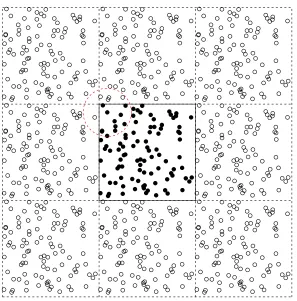
2.2.2 A virtual topography division . . . 43
2.2.3 Complex spatial windows . . . 45
2.3 Other issues in parallel computing . . . 49
2.3.1 Multiple layers of workers . . . 49
2.3.2 Optimal number of processors . . . 50
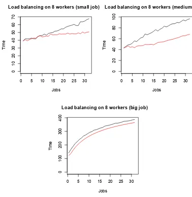
2.3.3 Load balancing . . . 51
2.4 A simulation model of optimal parallel computing structure . . . 54
2.4.1 A simple model . . . 54
2.4.2 A simple model with concurrent job distribution and load bal-ancing . . . 56
3 Parallel computing for spatial point processes 59 3.1 Edge correction methods . . . 59
3.1.1 Comparison of edge correction methods . . . 69
3.2 Parallel computation of point process summary functions . . . 70
3.3 Performance benchmarks . . . 75
3.4 Point process model fitting and evaluation . . . 77
3.4.1 Simulation envelopes . . . 79
3.5 Point process reconstruction . . . 80
3.5.1 The general reconstruction algorithm . . . 81
3.5.2 An improved reconstruction algorithm . . . 87
3.5.3 Parallelizing reconstruction . . . 89
3.6 The parspatstat package . . . 94
3.6.1 Function usage . . . 95
3.6.2 Datasets that do not fit in memory . . . 97
3.7 Example: Ontario lightning data . . . 98
4 Parallel computing for lattice models 109 4.1 Motivating example: Lattice Fire Spread Model . . . 109
4.2 Benchmarking and scaling issues . . . 110
4.3 Optimizations . . . 114
4.3.1 Time barrier . . . 114
4.3.2 Irregular division of lattice . . . 116
4.4 Parallel computing for Markov Chain Monte Carlo . . . 118
4.4.1 Multiple chain MCMC . . . 121
4.4.2 Single chain MCMC . . . 124
4.4.3 Continuous pre-fetching . . . 129
4.4.4 Comparison with other parallelization techniques . . . 131
5 Conclusion 132 5.1 Further Work . . . 133
Bibliography 135
Curriculum Vitae 140
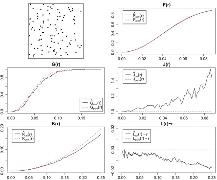
1.1 Summary functions plotted for a realization of a homogenous Poisson process with intensity λ= 100 in a unit window. The top-left graphic is a plot of the realized poisson pattern. . . 14 1.2 When looking at a search radius that lies outside the boundary of
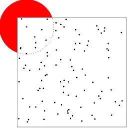
the spatial window, no points exist in this censored region (solid red), leading to a biased estimate of summary functions. . . 17 1.3 A manager-worker model for parallel computing where a single
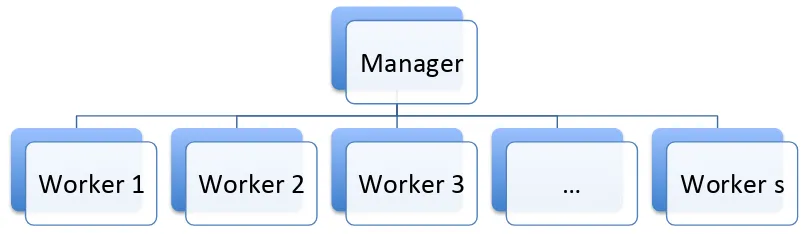
proces-sor (the manager) is dedicated to distributing work to and consolidat-ing results froms processors (the workers). Communication can occur between manager and workers but also between workers themselves in some circumstances. . . 24 1.4 Parallelizing multiple simulations by distributing independent
simula-tions to multiple CPUs. . . 29 1.5 Parallelizing a single simulation by distributing smaller dependent parts
to multiple CPUs. . . 29
2.1 Division of lattice from 1 to 9 processors, maintaining uniform sub-lattices. . . 46 2.2 Division of lattice from 1 to 9 processors, minimizing sub-lattice
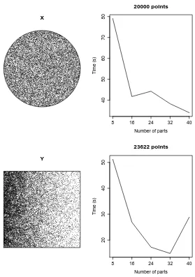
bound-aries. . . 47 2.3 Benchmark of the number of jobs vs computation time on two different
point patterns. . . 53 2.4 Benchmark of the number of jobs (in excess of the number of
work-ers) vs time with load balancing (red line) and without load balancing (black line) for varying data sizes. . . 58
3.1 Toroidal edge correction on a point pattern (solid points) by replicating the point pattern 8 times (hollow points) but only treating the original points as centers. . . 61
Only interior points (solid points) are used as centers. In this example, it resulted in 74% of points being discarded using a maximum search radius of 1/4 of the square window dimensions. . . 64 3.3 The border method may not work well for even a simple window shape
if it needs to be reduced by the some maximum search radius (left). It may result in disjoint interior windows if the maximum search radius is too large (right). . . 65 3.4 The plot of cells data (left) and its corresponding Fry plot (right). . . 67 3.5 Smoothed estimates of the reduced second moment measure, from
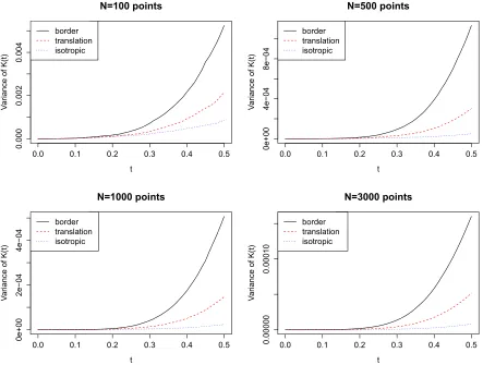
which an estimate of theK function can be obtained at varying radius distances from the origin. . . 67 3.6 Estimated variances from simulation of binomial processes with varying
n under border, isotropic, and translation correction methods. . . 71 3.7 A simple example of dividing a point pattern (above) into two
sub-windows (below). Although the spatial window is divided by half, points that are within the area covered by the maximum search radius (area enclosed by dotted red line) still need to be stored. . . 73 3.8 When applying edge correction in parallel computation of spatial
statis-tics, each processor is aware of only the extent of its own sub-window, yet needs to be aware of whether a boundary is a global boundary (black) and requires edge correction, or an interior boundary (red) that requires no edge correction. . . 74 3.9 Benchmark of the number of CPU vs time for uniform point process
patterns of varying size. . . 76 3.10 Speed up of parallel K-estimate for point patterns of varying sizes. . 77 3.11 The observed point pattern and a reconstructed point pattern (top).
Energy function of the reconstructed point pattern over 1,500 iterations (bottom). . . 85 3.12 The observed point pattern (left) and a balanced reconstructed point
pattern (right). . . 89 3.13 Comparison of simulation envelopes of K-function for the observed
point pattern, reconstructed point pattern, and a balanced reconstructed point pattern. Bottom graph shows the effect of a balanced algorithm in better matching at small values of r. The top and bottom lines of each colour indicate the upper and lower bounds of each envelope. . . 90
3.15 Chunking in a dataset and distribution to workers. . . 99 3.16 Map of all lightning strike data and the extent of the extracted spatial
window. The extracted spatial window is plotted with points intead of a + symbol and thus appears lighter. . . 100 3.17 Summary of Ontario lightning strike data from 1992 to 2010 by year
(top) and by month (bottom). . . 101
3.18 Plot of lightning strikes in a region of northern Ontario between 47◦ and 51◦ latitude and −84◦ and −80◦ longitude in 2003 (left) and 2008 (right). . . 103 3.19 Plot ofK-estimates of lightning strikes in a square region of Ontario in
2003 (top) and 2008 (bottom) using various border correction methods along with the theoretical line. . . 104 3.20 The original and reconstructed point patterns (top) and the
corre-spondingK-functions (bottom). . . 107 3.21 The original (left) and reconstruct point patterns (right) conditioning
on the points in red. . . 108
4.1 Simulation of a simple fire spread model with uniform wind on a 120x120 lattice. Red dotted lines represent division of sub-lattices to 4 CPUs. . . 111 4.2 Computation time of 48 fires distributed amongst 2 to 24 CPUs on a
1,200 by 1,200 pixel lattice. . . 113 4.3 Computation time of 48 fires distributed amongst 2 to 24 CPUs on a
240 by 240 pixel lattice. . . 113 4.4 Illustration of 3 CPUs working in parallel with communication only
when all three CPUs have hit a time barrier or requires swapping. . . 115 4.5 Illustration of 3 CPUs working in parallel with communication at every
time step to synchronize. . . 115 4.6 Buffer zone to alleviate communication due to boundary crossing, but
covers less total area. . . 119 4.7 Movement of a point (striped) from one processor to another location
(solid). The second processor (blue) does not actually receive the point until it passes the buffer zone. . . 120
draws are computed in four time steps. . . 123 4.9 Metropolis trees with prefetching two steps at a time using 3 processors.
At each time step, two levels are completed, representing two draws in the chain. Four draws are completed in two time steps. . . 125 4.10 Metropolis trees with dynamic prefetching where the most likely paths
are evaluated in parallel using 3 processors. At each time step, up to 3 levels are completed. In this particular example, five draws are completed in two time steps. . . 127 4.11 Comparison of speed-up versus serial MCMC from using up to 100
processors using simple pre-fetching and dynamic pre-fetching and two different targeted acceptance rates. . . 128 4.12 Metropolis trees with continuous prefetching where processors can be
assigned to higher levels paths to more quickly determine which path is correct and then processors can be reassigned down further down the most probable paths. Asterisks indicate cells that are being com-puted in parallel and purple cells indicate cells that are already under evaluation. . . 130
5.1 Splitting a three dimensional lattice into smaller sub-lattices. . . 134
Introduction
1.1
Spatial point processes
Spatial point processes form a large component of the field of spatial statistics. A
spatial point process, N, is a model that aims to describe an observed point pattern.
A realization or sample fromN is a point pattern consisting ofnpoints, each of which
has a spatial location in d dimensions attached to it.
x1, . . . , xn∈Rd
In the remainder of this thesis, Cartesian coordinates ind= 2 dimensions (the planar
case) are primarily used as the location measure, though other measures may be used
(e.g. polar coordinates). In practice, d is rarely greater than 3 since point processes
are usually used to describe a physical problem in up to three spatial dimensions.
A point pattern is observed within a spatial window, denoted E, which is a
sub-set of the space on which the process is defined, Rd. Often, the spatial window is
rectangular or circular in shape for the sake of simplicity but can technically be any
polygon. Complex polygon spatial windows arise in practice both naturally
(geo-graphic boundaries such as tree lines) and artificially (man made boundaries such as
roads or political divisions). There are situations where a spatial window can exhibit
an interior ‘hole’ or even an island within a hole. The number of points that exist in
an arbitrary window,W, is denoted by the functionN(W) while the volume (area) of
the same window is denoted by the function A(W). Thus, we haveN(E) = nthough
in practice, the number of points in a window is usually not fixed beforehand.
In addition to a location, each point in a spatial point pattern can also have one or
more measures attached, known as marks. These measures, the location themselves,
and correlation structure between points serve to characterize a point pattern through
summary statistics and functions, described in more detail in section 1.1.4.
that it is assumed that points exist in continuous space, though depending on the
sampling strategy of the data, these points may be discretized to a lattice structure.
Lattice structures need to be handled differently and will be discussed in more detail
in section 1.2. However, it should be noted that discretized data can be reduced to
a marked point process using smoothing techniques, as has been done in image pixel
analysis.
The second assumption is that we are only dealing with infinite point processes.
That is, it is assumed that the underlying model generating the point pattern extends
infinitely but we are only observing the points within a chosen spatial window, the
choice of which is made such that the point pattern is homogeneous within the window
or additional covariates are included to explain any heterogeneity that may exist.
A finite point process on the other hand, exists only within the spatial window
with the distribution of points within the window perhaps dependent on proximity
to the edge of the window. This is not to be confused with edge effects and edge
correction methods that are discussed in section 3.1 on infinite point processes where
1.1.1
Homogenous Poisson process
Before discussing the homogenous Poisson process, we will discuss the finite binomial
process. The finite binomial process is the simplest point process where n points are
distributed completely randomly in a given spatial window, E. The probability of a
pointxappearing in any interior windowW is uniformly distributed with probability
equal to the proportion of the area of W to the area of E:
P(x∈W) = A(W)
A(E) where W ⊂E.
When generalized ton pointsx1, . . . , xn, these points are independent and uniformly
distributed in E when for all interior windows W1, . . . , Wn,
P(x1 ∈W1, . . . , xn ∈Wn) =P(x1 ∈W1). . . P(xn ∈Wn) =
A(W1). . . A(Wn)
A(E)n .
To further generalize the binomial point process, we do not have to fix the number
of points in the point process, n. This leads to the homogeneous Poisson process if
the number of points is Poisson distributed with some intensity parameterλ per unit
area. Such a process is known as a completely spatially random (CSR) process where
(points appearing far from each other, also known as inhibition). The homogenous
Poisson process is often the “benchmark” that various simulation and assessment
methods use as a baseline comparison.
It should also be noted that the combination of many point patterns converges
in behaviour to a Poisson process by the Poisson convergence theorem [21]. Also, a
linear transformation of a Poisson process is still a Poisson process. In particular, if
N is a homogenous Poisson process with intensity λand B is a linear mapping, then
BN ={Bx:x∈N}is a homogenous Poisson process with intensityλ×det(B−1) [20].
1.1.2
Inhomogenous Poisson process
A homogenous Poisson process can be generalized to an inhomogenous Poisson process
where the constant intensityλis replaced by the intensity functionλ(x). The number
of points in a window B is Poisson distributed with meanRBλ(x)dxand the number
of points in disjoint windows are independent. The second property is known as
independent scattering. From a given point pattern, one can estimate the intensity
function using parametric methods such as maximum likelihood estimation.
To generate from an inhomogenous Poisson process with intensity function λ(x),
one can first generate from a homogenous Poisson process with intensity equal to the
used to determine which points should be deleted (thinned) until the desired
inho-mogenous intensity surface is met. This is done by rejecting a point with probability
equal to the proportion of its intensity to the overall maximum density.
The finite Cox process is a generalization of inhomogenous Poisson process where
the intensity surface λ(x) is random. It is a two stage process where a random
inten-sity surface is generated, and then an inhomogenous Poisson process is constructed
conditional on the generated intensity surface. This is also known as a doubly
stochas-tic Poisson process.
To determine if the intensity surface should be a random variable (that is, to
justify the use of a Cox process), multiple samples in the same window are necessary.
The intensity function can be estimated for each sample and compared.
1.1.3
Stationarity and isotropy
The concepts of stationarity and isotropy are important when dealing with point
processes since they are often assumed to be true when using the methods described
in this thesis.
A stationary point process, also known as an homogenous process, is a point
same regardless of how that window is translated. That is,
N +α=d N for all α∈Rd. (1.1)
where if N ={x1, x2, . . .} then N +α={x1+α, x2+α, . . .}.
A related concept to stationarity is isotropy. A point process is isotropic if it the
distribution of the number of points in a given window is the same regardless of how
that window is rotated. That is,
N=d RβN for all β whereRβ is a rotation of angle β.
The aforementioned homogenous Poisson process is both stationary and isotropic. In
other words, one would expect all sub-windows W ⊂ E that are the same shape to
exhibit the same spatial characteristics regardless of orientation and position in E
whereas an inhomogenous Poisson process would by definition be non-stationary.
1.1.4
Summary statistics and summary functions
Superficial characteristics of a point pattern such as clustering or regularity can often
characteristics, can be measured through summary statistics and summary functions.
The most basic summary statistic is point intensity, defined as the expected
num-ber of points in a unit area of the point pattern. This is denoted as λ with
corre-sponding estimator ˆλ, satisfying the following definition for the expected number of
points in an arbitrary spatial window W:
E(N(W)) =λA(W)
This intensity is often not known and the standard estimator is simply the number
of points in the observation window per unit area,
ˆ
λ= N(E)
A(E).
If counting the number of points inE is not possible since it may be too time
consum-ing, other estimators of ˆλexist such as the distance method [11] and the point-quarter
method [20]. Such methods also lend themselves to reconstruction applications,
dis-cussed in section 3.5. In the non-stationary case, the intensity is instead replaced by
an intensity surface, λ(x) with estimation often done using maximum likelihood and
Going beyond single numeric summary statistics are summary functions (often
functions of a search radius, r). Those summary functions that are all based on a
count of the number of points around a “typical point” can be referred to as Palm
characteristics. We use the notation
nx(r) =N(b(x, r)\{x}) (1.2)
to denote the number of points in the point process N that is within a circle (we are
concerned with d = 2 dimensions) of radius r centered at point x excluding point
x itself. Assuming stationarity, by equation 1.1, we can translate all points to the
origin, o, and study the characteristics of just no(r) in the resulting point pattern to
obtain measures for the original point pattern. Further examination of this is given
in section 3.1 where edge correction methods are discussed.
In a spatial point pattern, several descriptive statistics of this nature can be used
to describe the point process characteristics. These include first-order statistics such
as the empty space functionF(r), the nearest-neighbor distance distribution function,
G(r), and second-order statistics such as Ripley’s K-function [2] K(r), and the pair
correlation function, g(r). These, in addition to the combination of the F- and
For a given point pattern, these functions can be compared to the corresponding
theoretical function for the homogeneous Poisson process as an indicator of inhibition,
clustering, or lack thereof (complete spatial randomness). Their theoretical values for
the homogeneous Poisson process are also given.
First-order summary functions
The F-function, known as the empty space function, denotes the probability that an
area of radius r around a typical point contains at least one point, defined as
F(r) = 1−P(no(r) = 0) for r≥0.
The G-function, known as the nearest neighbour distance distribution function is the
distribution of distances of a typical point to its nearest neighbour, not including the
point itself, defined as
G(r) = P(no(r)>0) for r≥0.
Again, the origin is used assuming stationarity is satisfied. For the homogenous
Poisson process, one would expect F(r) =G(r). If the probability of having a point
around an arbitrary point is smaller than the typical distance of a nearest neighbour,
F(r) ≥ G(r) would be indicative of clustering. Lieshout and Baddeley defines a
measure, J, based on these two functions [47], defined as
J(r) = 1−G(r)
1−F(r) for r≥0 and F(r)≤1.
For this function, one would expect J(r) = 1 for a homogenous Poisson process,
J(r) ≥ 1 to be indicative of regularity, and J(r) ≤ 1 to be indicative of clustering.
It is important to note that a non-Poisson process can also result in J(r) = 1, that
is, J(r) = 1 is a necessary but not sufficient condition for showing a process is a
homogenous Poisson process [4].
Second-order summary functions
The first-order summary functions described above do not look beyond the nearest
neighbour, potentially ignoring a lot of information. Second-order statistics are based
on pairwise interpoint distances. Ripley’sK-function [32] is a second-order descriptive
statistic that is commonly used to measure homogeneity of spatial point patterns.
That is, to determine if a point pattern with n points that lies within a spatial
windowE ⊂R2 follows a spatially random process or if it is the result of a clustering
the assumptions of stationarity and isotropy, the function, λK(r), is the expected
number of points within a distance r of a typical point.
λK(r) =E(no(r)) for r≥0.
and by dividing both sides by the intensityλ, we obtain a definition of theK-function
K(r) = E(no(r))
λ for r≥0.
In a homogenous Poisson process, this is simply the area of the search circle,K(r) =
πr2. More points than expected, K(r) ≥ πr2, is indicative of clustering and less
points than expected, K(r)≤πr2, is indicative of regularity.
Related to the K-function is the L-function introduced by Besag [6] which is a
variance stabilized version of the K-function, defined as
L(r) =
K(r) π
1/2
for r≥0.
which has an added benefit of being easier to interpret becauseK(r) = πr2is the area
of the search circle with radius rso theL-function for a completely spatially random
visually examine the nature of the point process. Deviations from a horizontal line
are easier to spot than deviations from a diagonal [20].
Figure 1.1 shows the aforementioned summary functions plotted for a realization of
a homogenous Poisson process with intensityλ= 100 in a unit window compared with
the corresponding theoretical summary functions for a homogenous Poisson process.
The pair correlation function, g(r), is another second-order summary function
that contains the same information as the K- and L- functions but has advantages
for graphical interpretation. It is defined as
g(r) = k(r)
2πr for r≥0
where k(r) is the derivative of K(r). That is, it satisfies
K(x) =
Z x
−∞
k(t)dt.
The pair correlation function is the correction factor of a point xin b(x) (with
prob-ability λdx) and a point y in b(y) (with probability λdy) where x, y are distance r
0.00 0.02 0.04 0.06 0.08 0.0 0.2 0.4 0.6 0.8 F(r) r F(r)
F^raw(r) Fpois(r)
0.00 0.05 0.10 0.15
0.0
0.4
0.8
G(r)
r
G^raw(r) Gpois(r)
0.00 0.02 0.04 0.06 0.08
1.0 1.2 1.4 J(r) r J(r)
J^un(r) Jpois(r)
0.00 0.05 0.10 0.15 0.20 0.25
0.00
0.10
0.20
K(r)
K^un(r) Kpois(r)
0.00 0.05 0.10 0.15 0.20 0.25
−0.02
0.00
0.02
L(r)−r
L(r)−r
L^un(r)−r Lpois(r)−r
probability of both x in b(x) and y inb(y) is thus,
p2(r) =g(r)·λdx·λdy
so for large radius r, points are expected to be independent sog(r) approaches 1. In
a cluster process,g(r)≥1 since points x, y are correlated.
Higher order summary statistics have been developed as well, for example
Schla-ditz and Baddeley’s T function that looks at the number of r-close triples of points
per unit area [36]. There are also topological summary characteristics that make use
of methods from other areas such as graph theory. The connectivity function for
example,c(r), measures the number of disjoint components when circles of a selected
radiusRare grown around each point and the union of all circles are taken as
compo-nents. The actual measure itself is taken as the probability of a point distancerfrom
a typical point to be in the same component. Nearr = 0, the number of components
will be close to the number of points and this function approaches 0 monotonically
for increasing r.
Other examples include detecting outliers in point patterns by statistically
ana-lyzing marks assigned to each point through point-based indices. Gaps in the data
then analyzing the areas of the resulting cells created by the graph edges. In this
the-sis, we will primarily focus on first- and second-order summary characteristics with
a particular emphasis on Ripley’s K-function as these are the ones that are most
commonly used in practice.
Edge correction methods
When computing the summary functions defined above, they all involve looking at
a circle of some radius r around a given point, namely no(r). A complication arises
when a point is withinr distance from the boundary of the spatial windowE so that
part of the search circle lies outside of E where no points are observed (Figure 1.2).
We will illustrate this point further in section 3.1 by examining theK-function where
this censored data creates a biased estimate for which we need to use edge correction
methods. In fact, theK-function is independent of the shape of the study area when
edge effects are corrected for properly [10].
The uncorrected K-function estimate is known as the naive estimator where we
have
ˆ
K(r) = 1
λn n
X
i=1
ni(r) forr ≥0.
If we include a ‘buffer’ area around our window of interest for which data is collected
the additional labor involved [17]. Various edge correction methods are described and
compared in section 3.1. Also of interest is theJ-function, for which it was shown by
Baddeley that estimates of the J-function even without applying edge correction are
unbiased [2].
Other summary characteristics
In addition to the described nearest neighbour and intensity statistic, researchers have
also defined indices that can be used as summary characteristics.
The index of dispersion is a location-based index that measures the ratio of the
variance of the number of points to the mean number of points in enclosed spatial
windows of a certain size and shape. Pielou’s index of randomness is also based on
location of points and is a function of the random distance from a test point to its
nearest neighbour. These location-based indices extend well to marked point patterns
because they can be computed independent of the mark.
Point related indices are those that assign a mark to each point based on some
characteristic of the point in relation to the pattern as a whole. An example is
the aggregation index which marks each point with its nearest neighbour distance
and aggregates these marks over the entire set to get a measure of average nearest
neighbour distance. Related to the aggregation index is the degree of colocalisation
which is a function of some search radius r and gives the proportion of points that
have an aggregation index mark smaller than r. The mean direction index marks
each point by the sum of the unit vectors from the point to itsk nearest neighbours.
This gives the general direction that a point’s nearest neighbours are in. If a point
1.1.5
Point process model fitting and assessment
Given a point pattern, a common question of interest is whether or not the pattern
exhibits one or more characteristics of clustering, regularity, and randomness. Note
that it is possible for a point pattern to have short range clustering yet long ranger
regularity. To test this, we compute summary statistics of the point pattern and
compare that with the same summary statistic computed either on realizations of a
homogeneous Poisson process model or analytically on the theoretical homogenous
Poisson process model. If the results are statistically different in a two-sided test,
then it is evidence against complete spatial randomness. A one-sided test would
indicate either clustering or regularity. This result is necessary, but not sufficient proof
of complete spatial randomness and multiple tests are recommended. In practice,
functional summaries like theK-function or its variance stabilized version,L-function,
are used with the maximum point-wise difference with the same function computed
on a realization of the point process as an approximation to the theoretical value.
The advantage of comparing with realizations from a point process model is that
it can easily be extended to more complicated point process models as well since
theoretical values of many summary functions can only be analytically determined
for simple point processes. Beyond comparing observed point pattern characteristics
process models, which will not be discussed in detail here.
The choice of maximum search radius distance is important as well since variance
at larger radius will be high, thus weakening the power of the test. In order to account
for this, Ho and Chiu [19] proposes a modifiedL-test with a weight function for higher
search radii r. A comparison of the variance as a function of the choice of radius on
different edge correction methods is given in section 3.1.1 to demonstrate the larger
variance problem at larger radiuses.
A resampling method can be used as a means to assess the fit of a model as well.
Simulated realizations from a proposed model are generated and summary functions
are computed for each realization. Point-wise or global quantiles for these can be
used to construct an envelope to observe if the summary function for the observed
point pattern fits within this envelope. Further details for such methods are given in
section 3.4.
1.2
Stochastic lattice models
Stochastic lattice models are a way to represent spatial locations in a grid structure
where each cell (pixel) is in a state and evolves according to stochastic transition
of a forest fire front [7]. They are also used in statistical physics for modelling
ferro-magnetism, in biology for predator-prey models, and in epidemiology for modelling
disease transmission. The grid structure of the lattice model lends itself to take
ad-vantage of parallel computing. This parallelization allows us to decrease computation
time which can allow us to increase resolution of the lattice, work with a larger lattice,
decrease time step size in simulation, or work with a more complicated model.
Lattice models also have a direct translation to point processes models, notably,
a reason for studying lattice-based processes is their relatively tractability by
com-parison with inhibition processes [11]. Assuming each lattice cell represents a point,
then depending on how the position of a point is interpolated within a cell, this can
naturally produce inhibition between points. For example, if we take the centre of
each cell as the location of a point, then a hardcore inhibition distance equal to the
cell dimensions will exist.
1.2.1
Markov random fields
Markov random field models were first introduced in 1974 by Besag [5] and were
intended as a stochastic model to describe spatial processes of points represented
in a lattice. A set of random variables are organized in a lattice structure so that
that the functional form ofP(xi|x1, . . . , xi−1, xi+1, . . . , xn) is dependent uponxj. In a
square lattice structure, this creates a possible first-order neighbour structure of cells
consisting of cells immediately to the top, left, right, and bottom of an existing cell.
The value for a cell is dependent only on its neighbour cells. Higher order neighbour
structures can be defined to extend beyond immediate neighbours as well but we will
mainly look at the first-order neighbour structure as it is the most common.
Techniques discussed in Chapter 4 can be directly applied to a Markov random
field existing on such a lattice structure if we wanted to simulate a stochastic
realiza-tion. If we wish to analyze a Markov random field, doing so by direct calculation is
very difficult. Even for an unrealistically small 40 x 40 pixel image where the pixels
take on binary values, there are 21600 = 4.4× 10481 terms in the summation [15].
Using a Bayesian approach, one can employ Markov Chain Monte Carlo (MCMC)
techniques such as those described by Givens and Hoeting [15] to do so. A description
of MCMC and techniques for parallelizing MCMC are given in section 4.4.
1.3
Parallel computing
For the past several years, computing power has plateaued due to physical constraints
computing power. Instead, parallel computing, which uses multiple processors to work
concurrently to speed computation, has been the focus of research and development in
recent years. From a statistical computing perspective, high-performance computing
(HPC) that makes use of computer clusters consisting of thousands of cores is one of
the primary tools to compute intensive simulations and calculations.
Two architectures of parallel computing are multithreading and multiple
process-ing. The main difference between multithreading and multiple processing is the
mem-ory architecture. Multithreading involves dividing a single process into the work of
multiple computing threads. Each of these threads share the same memory
architec-ture and usually exist on a single computer system. Multiple processing on the other
hand divides a problem into smaller problems that are then worked on independently
by separate processors. Each processor sees only its own memory structure and if
required, can exchange information with other processors. Multithreading provides a
simpler method of parallelizing problems due to all threads working on the same data
(equal access to shared memory) but is limited in the amount of speed-up possible
for memory intensive computations. Multiple processing can scale linearly (ignoring
communication overhead) with the number of processors used but is more complicated
to implement. Although communication overhead will always exist, it can be
this paper, multiple processing is the primary focus though there is room to use
mul-tithreading within the computation of individual processors such as parallel matrix
computations implemented by libraries that can take advantage of multithreading.
In this thesis, we will be using a manager-worker model for parallel computing
where a single manager processor is dedicated to distributing work to and
synchro-nizing any number of worker processors (Figure 1.3). Although workers mostly
com-municate with the manager, it is possible for workers to directly comcom-municate with
one another to avoid having a communication bottleneck at the manager level. Most
problems will have one layer of workers although technically each worker can in turn
be a manager with its own set of workers. For example, we may wish to accommodate
large datasets at each division of workers. Such a multi-layer division is described in
section 2.3.1.
Manager
Worker 1
Worker 2
Worker 3
…
Worker s
1.3.1
Hardware specifications
In this thesis, simulations were carried out on themakocluster on the shared
hierar-chical academic research computing network (SHARCNET). This particular cluster
contains only 244 cores and is rarely used relative to larger clusters with thousands
of cores. It is meant for development and testing purposes so each job has a one-hour
limit on run time. Such an environment is not ideal for running actual analyses that
may require longer run time but is suitable for performing benchmarking tests on a
varying number of processors. However for this same reason, the “wall clock” time
of jobs was kept to under an hour when run on a single processor so that the exact
same computations can be run on multiple processors and their results can be fairly
compared. In this thesis, the terms cores, processors, and CPUs are used
interchange-ably to denote the number of individual central processor units utilized in a parallel
system.
The cluster runs on CentOS 5.2 and consists of four types of nodes: 1
adminis-trative node, 1 login node, 14 Xeon computation nodes and 16 Nehalem computation
nodes. Care was taken to carry out all benchmarks on only one type of node (Xeon
nodes, in this case) to ensure uniformity between hardware. Nodes are interconnected
through gigabit ethernet and jobs were kept to as few nodes as possible to minimize
operating at 3.0 GHz with 8GB of memory per node.
1.3.2
Parallel programming in R
R is an open source implementation of S, a programming language for statistical
computing and graphics [31]. It is widely used both in practice and research in
many fields across industry and academia. The core R software is supported by an
active development team while external libraries that extend the functionality of R
are developed and maintained by the community. As of writing, there are currently
over 4,2800 of these external libraries, known as packages, on the Comprehensive R
Archive Network (CRAN).
Support for parallel computing has been available in R for some time,
Schmid-berger et al. provides an excellent state of the art review [37]. Of note are two packages
on which many of the existing parallel computing packages are built: multicore [44]
and Rmpi [50]. To summarize, themulticore package allows for single computers to
make use of all available cores on the machine, commonly two to eight cores, while
Rmpi is designed to work on computing clusters with many cores spread out across
many machines (nodes), though it is also capable of being run on a single computer
with multiple cores. The widely usedsnow package [45] can extend theRmpipackage
Versions after R 2.14.0 include theparallelpackage [30] as one of the base
pack-ages in R. This package is a derivative of multicore and snow to further simply the
end user’s process of adapting their code to take advantage of parallel programming.
A more recent package, pbdMPI [26], focuses on “pretty big data” using the MPI
framework. The idea here is to have each worker process perform computations on its
own portion of a data set without the necessity of a managing computer controlling
their behaviour. The advantage of this is allowing enormous data sets to be used since
the data set does not need to be transferred to each worker individually. Individual
results from workers can then be aggregated together to get the desired final result.
However, this package assumes the problem is embarrassingly parallel, as described
below.
1.3.3
Embarrassingly Parallel and Non-embarrassingly
Par-allel Problems
When applying parallel computing to statistics, problems can be divided into two
groups: embarrassingly parallel problems and non-embarrassingly parallel problems.
Embarrassingly parallel problems consist of running multiple independent
processes and then results are combined at the end (Figure 1.4). They are known as
embarrassingly parallel problems due to how simple it is to conceptualize and in many
cases, implement. In fact, all of the aforementioned parallel packages were developed
for the embarrassingly parallel problems and are relatively straightforward to use.
In fields like spatial statistics, a problem may arise where computation on one
location of our spatial dataset may be dependent on the concurrent computation of
another location in our spatial dataset. This dependency requires workers to
commu-nicate with one another in an efficient way without creating long stalls in computation.
These are referred to as non-embarrassingly parallel problems. An example of this
is when we wish to apply parallel computing to a single large simulation of a lattice
model. We can divide the lattice into smaller sub-lattices and then have each
proces-sor perform computations on a single sub-lattice (Figure 1.5) but we need to maintain
communication between processes that are responsible for adjacent sub-lattices.
Specific issues that arise when parallelizing computation in spatial statistics are
CPU
Sim Sim
Sim Sim Sim Sim
Sim
CPU
CPU
CPU Sim
Sim Sim
Sim Sim
Sim Sim
Figure 1.4: Parallelizing multiple simulations by distributing independent simulations to multiple CPUs.
CPU
Sim
Sim Sim
Sim
CPU
CPU
CPU Sim Sim
Sim Sim Sim
1.4
Motivation for parallel computing in spatial
statistics
This section serves to give an overview some of what has been done in parallel
com-puting applied to various areas of spatial statistics as well as examples of applied
statistical work that could potentially take advantage of the methods introduced in
this thesis.
1.4.1
Use of spatial statistics in different disciplines
In ecology, Hasse [17] gives an overview of how to use theK-function in an ecological
setting along with descriptions of edge correction methods. The methods were applied
to both a real scrubland dataset and a computer generated dataset. Notably, he finds
that the most effective edge correction methods are also the ones that have the highest
computational requirement and points out shortcomings of the border method and
toroidal correction. He also notes the non-standardized implementation of statistical
analysis methods by other researchers that are not easily reproducible as many of the
computer programs are either developed by the researchers themselves or modified
programs from colleagues. One goal of this thesis is to provide an open-source library
used and even built upon by anyone.
In forestry, Szwagrzyk et al. [43] examined the spatial distribution of trees in
East-Central European forests using the K-function with edge correction done using the
border method in a circular spatial window. This was compared with the theoretical
homogenous poisson model to determine if clustering or regularity exists. In their
analysis and other analyses of a similar nature with which they compared results, all
were done on a small spatial scale which give a very manageable number of points
to work with. The resulting methods from this thesis aims to alleviate compromises
that need to be made with regards to size of datasets. Stoyan and Penttinen [41]
gives an excellent summary of how spatial point process methods have been used in
various aspects of forestry, including the calculation of summary characteristics, the
reconstruction of point patterns, and stochastic models for marked point patterns.
1.4.2
Parallel computation in spatial statistics
A lot of the research that has been published on the use of parallel computing in
spatial statistics has been from a geography standpoint. This is unsurprising as
geography is a large area where spatial statistics has been used for many years. In
1990, Griffith [16] discussed limitations to spatial statistics at the time, which were
geographic data sets outpacing the numerical computation capabilities at the time.
He notes the importance of developing statistical algorithms with parallel computing
in mind to take advantage of scalable computational resources.
In 1995, Armstrong and Marciano [1] looked at the parallel computation of a
measure of spatial association introduced by Getis and Ord in 1992 [14]. Here, they
examined the algorithm used for computing the measure to identify bottlenecks that
are computed serially. They implemented portions of the algorithm in parallel and
noted that the performance gain with parallel processing increase with the size of the
data. Likewise, computation time increases at a slower rate in a parallel
implemen-tation compared to a serial implemenimplemen-tation across datasets of equal size. This agrees
with conclusions drawn throughout this thesis.
For lattice models, Cannataro et al. [9] developed a software environment for the
parallel modelling of cellular automata models where cells (pixels) evolve according to
transition rules that are dependent on its immediate neighbours. They examine the
hardware required to run such a model in parallel, separating the system design into
graphical and computational components. Load balancing from distributing work
evenly across processes was also considered but this only applies when the model is
dependent on first order neighbours. There are other strategies for optimizing parallel
1.5
Outline of Thesis
The rest of this thesis is divided into a further four chapters. Chapter 2 will give an
overview of both general issues and issues specific to parallelizing spatial statistics
that will be encountered. Chapters 3 and 4 give methods and examples of applying
parallel computing to spatial point processes and stochastic lattice models
respec-tively. These chapters also look at performance benchmarks and introduce novel
methods for further optimization. The package that accompanies the methods
de-scribed is also introduced here along with examples on real data. Finally, Chapter 5
is the concluding chapter with discussion of further work and natural extensions to
Issues in parallel computing
2.1
Issues with Parallelizing Single Simulations
As mentioned in section 1.3.3 regarding non-embarrassingly parallel problems, there
are computational issues that arise when dealing with sub-problems that are
depen-dent on results or information from adjacent sub-problems. These issues include the
actual programming implementation as well as computational bottlenecks that need
to be considered.
2.1.1
Message Passing Interface
Communication between processors (CPUs) in parallel programming is accomplished
by message passing. Message passing is a programming paradigm used widely on
parallel computers, especially Scalable Parallel Computers with distributed memory
and on Networks of Workstations [39]. Message Passing Interface (MPI) has been
the standard specification for message passing libraries across many computing
plat-forms. It specifies a framework of functions that can be used for communication
between processors regardless of hardware implementation. The Rmpi package is the
R interface for the MPI framework [50], which serves as a wrapper for the underlying
MPI implementation such as MPICH2, LAM/MPI, and OpenMPI. The Rmpi
pack-age is commonly required by various packpack-ages that wish to take advantpack-age of parallel
computing in R. In this thesis, this package is built upon and widely utilize on top of
OpenMPI, though it will work with other MPI implementations as well.
2.1.2
Random number generation
In stochastic models, properly generated pseudorandom numbers are a necessity.
Se-quences of pseudorandom numbers are generated based on a seed that is often a
a deterministic algorithm and consists of a finite sequence of numbers that appear
to be random, hence they are called pseudorandom. One can imagine that all CPUs
running on the same system would read the same system time and hence generate
the exact same sequence of random numbers. This would of course not be ideal if we
wish to simulate a stochastic system where it is assumed that random number inputs
are independent. In fact, in order for each worker to have an independent stream of
random numbers, the period of a random number generator should be much larger
than the total number of random numbers required by all workers so there is no
over-lap in the random number streams. Random number generation is taken care of by
the rlecuyer R package to ensure that each CPU has a proper stream for a given
seed. As of R 2.14.0, the parallel package in R incorporates the L’Ecuyer-CMRG
random number generator so explicit use of the rlecuyer package is not necessary.
For the purposes of this thesis, it is assumed that non-indendence of pseudorandom
number streams is properly dealt with.
A further issue arises when we wish for our results to be reproducible.
Tradi-tionally, setting the initial seed will result in the same sequence of pseudorandom
numbers and hence the same results from running a simulation. However, in a
paral-lel computing context, multiple processors will be working on the same job and even
in hardware and other external factors, different processors may work at different
speeds. For example, consider a large simulation that is divided into smaller pieces
and multiple processors compute these pieces one at a time on a first come first serve
basis. Processors may take these pieces in a different order each time depending
on the order that computation finishes. On a different system even with the same
number of processors, this order that processors compute pieces in may not be the
same if group of processors are faster or if the network communication is different.
Hence the original results may not be reproduced. In order to account for this, one
can keep track of the order in which the processors compute pieces and enforce this
in subsequent simulations if one wishes to reproduce simulation results. However,
if a job that was originally completed quickly by a fast processor is assigned to a
slow processor in a new system, the entire job queue will be held up while this job
completes. Another solution is to force synchronization so processors cannot move
onto the next piece until all processors have completed, at which point chunks can be
distributed in some predetermined order. This also has the issue of faster processors
sitting idle waiting for all other processors to complete their computations. Neither
solution will give optimal speed-up and thus reproducibility is enforced only when it
2.1.3
Workload distribution
Depending on how the processors are allocated and the complexity of the problem in
each sub-problem, there could be an uneven (suboptimal) distribution of workload.
Some processors may be idle while other processors may be doing all of the work.
Some load balancing can be done but we will introduce several ideas to minimize
in-efficiencies in the workload distribution. The goal is to have all processors finish their
computation at roughly the same time whilst minimizing the amount of
interproces-sor communication required. One complicating factor in workload distribution is the
uniqueness of different hardware systems since the optimal distribution of workload
depends heavily on the architecture of the system that it is running on. For example,
specially designed computing clusters may have extremely low interprocessor
com-munication that is minimized through the use of specialized hardware switches while
distributed clusters may have a high number of processors but intercommunication
may be several orders of magnitude higher. As such, the trade off between the size of
each problem and the amount of communication required between processors needs
2.1.4
Example: Two-dimensional Heat Diffusion System
To motivate the idea of parallel programming on a lattice and to demonstrate some of
the issues described above, we can consider a two-dimensional heat diffusion problem.
At a given timet, the change in heatutis defined as a function of neighbouring values
ut=a(uxx+uyy)
with ut representing the partial derivative and uxx and uyy representing the second
partial derivatives of the temperature function u(x, y, t). At time t = 0, the initial
value at a specific coordinate (x, y) is determined by some predefined function φ.
u(x, y,0) =φ(x, y)
Using a finite difference method we can implicitly solve for the value of each lattice
pointvi,j as only a function of the value of neighbouring lattice points at the previous
time step:
vni,j+1−vni,j
∆t =a
vn
i+1,j−2vi,jn +vni−1,j
∆x2 +
vi,jn+1−2vi,jn +vni,j−1 ∆y2
vni,j+1 =vi,jn +a∆t
vn
i+1,j −2vni,j+vi−n 1,j
∆x2 +
vni,j+1−2vni,j+vi,j−n 1 ∆y2
In order to parallelize this example, we can divide the lattice into a number of
sub-lattices equal to the number of processors we wish to use and distributed as such.
Since initial values are not dependent on neighbours, each processor can determine
the initial value of each coordinate in its sub-lattice. To compute the next time step,
all the points in the lattice are traversed. If the point is an interior point, that is,
all of its neighbours are fully contained within the sub-lattice, then computation can
be done independently. If the point is an exterior point whose neighbour exists in
another sub-lattice (not an overall boundary point), then communication is required
with the adjoining processor. In fact, information needs to be swapped in both
direc-tions at once in this example as the adjoining processor will have points that require
mirroring information. As one obvious optimization, the information swapping
be-tween processors can take place all at once with the entire boundary swapping in one
communication step as opposed to swapping information on demand. However, since
every point needs to be computes at every time step, communication must occur at
every time step. An example where communication need not occur at every time
step is given in chapter 4. Other discretization methods such as a hexagonal lattice
communication necessary between processors in order to do the computation. In a
hexagonal lattice, such communication requirements will only be exacerbated with
cells having more neighbours.
2.2
Issues in Parallel Computing of Spatial
Statis-tics
When dealing with spatial statistics and point patterns in particular, there are unique
issues that arise when attempting to parallelize existing algorithms both in terms of
hardware constraints, as well as mathematical considerations.
2.2.1
Memory limitations
In spatial statistics, point patterns can be represented in at least two ways: as a list
of coordinates or as a rasterized grid. Depending on the sparsity of the pattern, one
method may be more manageable than the other in terms of memory required to
store the point pattern. Section 3.6.2 deals with large data sets that do not fit in
memory.
A larger memory issue arises when computing summary statistics such as Ripley’s
from 0 to the maximum search radius R. R can be arbitrary chosen, but is usually
a function of the size of the observation window E. In order to account for edge
corrections when applicable, it is far more efficient to store a matrix of distances
(often Euclidean distance) from each point to all other points within R units as
opposed to performing pairwise distance measures every time it is required. However,
this computation requires allocating a matrix of sizen×n where n is the number of
points in the point pattern. As one can imagine, this does not scale well for large
point patterns, although if R is relatively small, then the pairwise distance matrix
can be quite sparse.
There are several ways to bypass this problem. One way to bypass the memory
limitation is to randomly sub-sample from the entire point pattern to reduce the
number of points we need to deal with. This will require some information to be
thrown out in a trade off for a more manageable computation. In fact, multiple
samples may have to be taken to ensure consistency in the measurements.
Another method to bypass the memory limitation is to use an approximate
algo-rithm. One such algorithm utilizes a fast Fourier transform to approximate the second
order K-statistic estimate done with a guard-area (border) edge correction method.
This too requires throwing out information near the border of spatial windows
translation correction. These edge correction methods are discussed in more detail in
section 3.1. A way to bypass the memory limitation without having to discard
infor-mation or resort to approxiinfor-mations is to take advantage of parallel programming and
simply scale the algorithm to work on computing clusters than can scale the memory
limit linearly while decreasing computing time sub-linearly.
First-order statistics like the G, F, and J-functions are not computed based on
pairwise distance measures between all points and thus do not have this memory
limitation issue but improvements can still be made to take advantage of parallel
computing if the data set is too large for a single computer to handle.
2.2.2
A virtual topography division
When using parallel computing, one would wish to divide a given spatial window into
smaller spatial windows so that each processor only needs to deal with a manageable
number of points. In single pixel algorithms where each pixel is not dependent on
any other pixel, this division is trivial as there would be no communication required.
However, more commonly, applications may require a processor to gather
informa-tion from neighbouring windows so a virtual topography must be maintained by all
processors to ensure proper communication.
the simplest division is to divide a spatial window into strips in one direction so that
each processor will only need to deal with two adjacent neighbours (one for edge
cases). However, in applications where communication between processors may act
as a bottleneck, long narrow strips may increase the number of times we need to
“cross boundaries” and perhaps even communicate with processors more than one
step away if the neighbourhood radius is large. Assuming communication does not
favour one direction, a better division may be one that more closely divides the
spatial window into square sub-windows with points centred near the middle of these
virtual divisions. That way, it may minimize the probability of a processor requiring
information swapping with a neighbour.
Mineter [18] describes two methods for partitioning a lattice for extent-based
algorithms, that is, algorithms that require pixels to know the state of other pixels
either in a limited local neighbourhood or even globally. The first is a partitioning
scheme that balances sub-window shape and number of messages. The number of
messages passed is kept low by ensuring corners are shared by either 2 or 4
sub-windows and shapes are kept uniform across all processors (Figure 2.1). As a result,
each sub-window will have a maximum of 4 neighbours. The second method known
as heuristic partitioning is to minimize the border lengths of each sub-window which
sub-windows, non-uniform sub-window shapes, and sub-windows with more than 4
neighbours (Figure 2.2). As can be seen, notable differences arise specifically on
a prime number of processors where the topography cannot be divided into n ×
m grids where at least one of n, m > 1. For our purposes, we will maintain
sub-lattice uniformity to ease coordination of communication between processors. This
is generally not a big issue as one can choose a number of workers to use to create
a lattice division with minimum boundary lengths (i.e., n2 processors where n is a
positive integer).
Once we get into more complex gridded topographies (more than nine processors),
each processor will have up to eight adjacent neighbours – four that share an edge,
and four that share a corner – all of which may be required to communicate with
each other depending on how the neighbourhood structure is defined.
2.2.3
Complex spatial windows
In some applications, we may have spatial window boundaries that are complex to
represent. For example, coastlines and natural or political boundaries on maps may
not always consist of straight line edges. These complex spatial windows may be
more easily represented as a binary mask on a lattice. In a binary mask, lattice
pixels with a majority of cover outside the region is indicated by a 0. Points are
also discretized in the same way depending on which pixel they fall into. Points that
are close together may end up in the same pixel and are either lost or counted as a
mark on the particular pixel. An obvious limitation of a discretized point pattern
is the loss of information, which can be mitigated to a certain extent depending on
the resolution of the lattice that is chosen. However, one should keep in mind that
a larger resolution (finer detail) will result in many of the same issues that were
discussed previously. A less obvious complication that may arise is when thin areas
may be discretized into disjoint islands if sufficient detail is lost. Entirely enclosed
islands (either natural or created through discretization) that are disjoint from the
rest of the spatial window also adds another layer of complexity when parallelizing.
Even assuming uniform behaviour between islands and the rest of the spatial window,
special care needs to be taken to ensure that spatial window divisions account for the
2.3
Other issues in parallel computing
2.3.1
Multiple layers of workers
Often times, we may wish to repeat a simulation multiple times to ensure consistency
or for estimation purposes. An excellent example of this is estimating envelopes
by simulating a random dataset many times and looking at certain quantiles (as
described in section 3.4). This type of problem is embarrassingly parallel since the
simulations are independent. However, if each individual simulation requires parallel
processing (due to memory limitations for example), then we require parallelization
at two levels. Care needs to be taken to set up the workers in such a way that each
worker is aware of which manager processor it needs to communicate with. This is
done using individually assigned communicators.
A map-reduce scheme is used to compile results from workers to a intermediary
node. A map-reduce scheme is where a problem is ‘mapped’ to multiple processors for
computation and then each will send results back to be reduced into a single solution.
These intermediary nodes then compile their results in another map-reduce scheme
to the manager processor (or depending on the complexity of the problem, another
set of intermediary nodes). This type of design can scale indefinitely but the number