A quantitative dynamic systems model of health-related quality of life among older adults

(1)

Clinical Interventions in Aging

Dove

press

O r I g I n A l r e s e A r C h

open access to scientific and medical research

Open Access Full Text Article

A quantitative dynamic systems model of

health-related quality of life among older adults

Correspondence: Mattia roppolo Department of Psychology, University of Torino, Via Verdi, 10, 10124 Torino, Italy Tel +39 011 6702 788

Fax +39 011 6702 791 email mattia.roppolo@unito.it

Journal name: Clinical Interventions in Aging Article Designation: Original Research Year: 2015

Volume: 10

Running head verso: Roppolo et al

Running head recto: Dynamic systems model of HRQOL DOI: http://dx.doi.org/10.2147/CIA.S91605

Mattia roppolo1,2

e saskia Kunnen2

Paul l van geert2

Anna Mulasso1

emanuela rabaglietti1

1_{Department of Psychology, University}

of Torino, Torino, Italy; 2_Department

of Developmental Psychology, rijksuniversiteit of groningen, groningen, netherlands

Abstract: Health-related quality of life (HRQOL) is a person-centered concept. The analysis of HRQOL is highly relevant in the aged population, which is generally suffering from health decline. Starting from a conceptual dynamic systems model that describes the development of HRQOL in individuals over time, this study aims to develop and test a quantitative dynamic systems model, in order to reveal the possible dynamic trends of HRQOL among older adults. The model is tested in different ways: first, with a calibration procedure to test whether the model produces theoretically plausible results, and second, with a preliminary validation pro-cedure using empirical data of 194 older adults. This first validation tested the prediction that given a particular starting point (first empirical data point), the model will generate dynamic trajectories that lead to the observed endpoint (second empirical data point). The analyses reveal that the quantitative model produces theoretically plausible trajectories, thus providing support for the calibration procedure. Furthermore, the analyses of validation show a good fit between empirical and simulated data. In fact, no differences were found in the comparison between empirical and simulated final data for the same subgroup of participants, whereas the comparison between different subgroups of people resulted in significant differences. These data provide an initial basis of evidence for the dynamic nature of HRQOL during the aging process. Therefore, these data may give new theoretical and applied insights into the study of HRQOL and its development with time in the aging population.

Keywords: older adults, dynamic systems model, nonlinear equations, simulated trajectories, validation

Introduction

It is well known that everywhere in the Western world, and particularly in Europe, the population is growing older.1_{From an individual point of view, consequences of the}

aging process are 1) health decline,2,3_{2) loss of autonomy,}4_{and 3) institutionalization.}4–6

From a societal point of view, health decline and loss of autonomy translate into an increase in direct (ie, health system) and indirect (ie, loss of productivity for caregivers) costs.7–12_{The increasing costs stimulate policy makers, practitioners, and researchers}

to find effective and low-cost solutions to reduce age-related expenditure.

Within this context, the evaluation of subjective assessment (ie, self-rated health) is considered increasingly important by researchers and clinicians, because it gives fundamental information about the processes that may affect a person (ie, drug administration, diseases). The use of health-related quality of life (HRQOL) indica-tors makes it possible 1) to monitor individual trends of health status and perceptions, and 2) to point out the achievement of specific health objectives in research (ie, implementation of innovative intervention strategies) and public health (ie, preven-tion campaigns).13

Clinical Interventions in Aging downloaded from https://www.dovepress.com/ by 118.70.13.36 on 20-Aug-2020

For personal use only.

Number of times this article has been viewed

This article was published in the following Dove Press journal: Clinical Interventions in Aging

(2)

Dovepress

roppolo et al

However, although the evaluation of HRQOL appears to have many advantages, the use of HRQOL indicators (espe-cially in hospitals and medical centers) is still limited, and as a consequence, knowledge concerning HRQOL processes has little influence on clinical decision making.14

The limited use in clinical practice may be related to the still prevailing lack of consensus among the available HRQOL models and instruments.15_{In fact, several authors include}

different domains in their HRQOL conceptualization.16–18

Diversity in theoretical models is also reflected in too many and diverse instruments.

In an attempt to overcome the diversity in models and instruments, Roppolo et al19_{analyzed various}

per-spectives (ie, demographic changes, health costs, and aging theories) and aspects (ie, health decline in different functional domains) related to the self-rated health in the aging process. In particular, some key aspects of HRQOL were highlighted, such as 1) its three-dimensional nature, starting from the World Health Organization’s definition of health,20_{which assumes health as a complete physical,}

mental, and social state of well-being, and 2) the twofold way of assessment (called here self-reported health status and experienced-health indicators) for each component, as proposed by Testa and Simonson.21_{Furthermore, a new}

conceptual model based on the theory of dynamic systems was outlined to highlight that HRQOL 1) should be regarded as a dynamic construct (ie, a phenomenon that can undergo changes during time), 2) could be viewed from a develop-mental perspective, that is to say, each step is the starting point of the following one, and the continuous iterations on a short timescale (ie, daily) are associated with long-term development (ie, monthly or yearly developmental trends), 3) may have domains connected to one other, indicating the inadequacy of direct and simple causal relations, 4) is subjected to random influences not directly assessable. This conceptual model delineated possible complexity and dynamic aspects of HRQOL, particularly in the aged population.

Starting from this approach, it will be possible to con-ceptualize, measure, and analyze HRQOL developmental trajectories in the older adults’ population making fundamen-tal steps to understand the role of aging process in self-rated health and to prevent health decline at an early stage, imple-menting health promotion interventions and strategies.

In order to obtain information about trends of changes in HRQOL, it is necessary to test theoretical assumptions in an empirical setting. A first step toward this aim is to build and conceptually test mathematical models that can

reproduce and predict empirically found developmental trends of HRQOL. Mathematical models represent mecha-nisms of development, and therefore, they can be used to test qualitative and quantitative properties of the process under study. Furthermore, a mathematical model is a good tool to test, simulate, and receive information about a system.22,23

Dynamic system models are not data-focused in the statistical sense of the word (they do not represent statistical associa-tions among patterns of empirical data, such as structural equation models), but they describe mechanisms of the sys-tem studied. Furthermore, these models are dynamic because they describe how one state of the system (intended as the state of an individual person) changes into another state of the system over the course of time.22,23_{A mathematical dynamic}

systems model of a developmental process includes 1) the concepts that are considered to be important for understand-ing the temporal course of the process, and 2) the dynamic relations between those concepts that are theoretically expected. These relations are translated into mathematical equations. The mathematical translation makes it possible to simulate the process under study. In other words, the model shows what happens over time in different conditions, with the possibility to test whether theoretical assumptions con-cerning the process are valid.22

It is relatively uncommon in social and psychological sciences to develop theory-based dynamic models. These models are capable of explaining change, explicitly specify-ing how one state of the system changes into another state of the system over the course of time, for all possible states that the system can occupy, in a way that generates a description of actual trajectories of change. Such models have various advantages such as the possibility 1) to take into account a large number of phenomena under study, 2) to analyze the structure of a system and its development during time, 3) to express types and directions of connections among domains, 4) to develop the model into a simulation tool, in order to test different situations and compare simulated results with empirical ones. In this way, a mathematical model may result in a better understanding of the phenomenon under study and may bring new knowledge to the specific sector of investigation.22

The dynamic systems conceptual model contributes to the conceptualization of HRQOL, integrating health domains, self-report health status and experienced-health components, stable individual parameters, and random influences.19

Theoretical assumptions include the choice of variables and domains, and the notions of how they affect each other. In order to test the validity of the theoretical assumptions, it is

(3)

Dovepress Dynamic systems model of hrQOl

necessary to translate the conceptual model into a mathemati-cal model that will be analyzed and validated.

The mathematical model reflects theories of HRQOL, in accordance with the use of the three main domains of health, and the adoption of a self-report health status and experienced-health components for each domain,20,21_and

represents the conceptual model as a dynamic system, reproducing its structure and connections. The reason to translate the conceptual model into a mathematical one is that it offers the possibility to express theoretical assump-tions and relaassump-tions in a quantitative/numerical form.22,24_The

advantages are related to the possibility to test hypotheses and compare simulated (based on the assumptions made in the conceptual model) and empirical data. Furthermore, the dynamic systems model allows one to analyze and represent differences among groups starting from different sets of initial and parameter values and to simulate perturbations (eg, a physical trouble) in the systems, in order to test its reactions to perturbations in life.

Once built, the model will be tested and validated with empirical data, in order to analyze the goodness of fit. The validation of the model is a mandatory step, because the sys-tem is based on the assumptions about the relevant variables acting on different time levels (ie, day-to-day level). The model will be able to simulate developmental trajectories of HRQOL, because it is assumed (starting from the conceptual model) that HRQOL is an iterative process. Iterative means that the process is reproduced again and again on a daily basis. The outcome of each day (each calculation in the mathematical model) is the starting point of the next day (next calculation). The equations in the model describe how the different variables affect each other on the level of one iteration, thus how they change, influenced by all components in the model, from one day to the next.22

The aim of this article is to make a first step in the valida-tion procedure by 1) translating the conceptual model into a mathematical model, taking into account all the specifics and features of the theoretical assumptions; 2) testing the model, to assess whether it produces theoretically acceptable trajectories; 3) comparing empirical and simulated data.

The conceptual model was conceived and designed spe-cifically for the aged population, but it can be adjusted to other target populations. It is composed of the following:

• Three main components (called growers, for their ability to change over time), namely the physical (P), mental (M), and social (S) domain of health. Each domain is seen as a subsystem, composed of self-reported health status and experienced-health indicators.

• A component that consists of stable individual para-meters. The stable individual parameters are age, presence of diseases, and presence of protective or risk factors.

• A random influence (stochastic part of the model) that directly acts on the three growers, and that is seen as a comprehensive term for the variety of unpredictable life events.

• A parameter (called adaptability) regarding the individual’s ability to cope with random fluctuations or internal and external stressors. This parameter is a direct representation of interindividual differences, and it will act directly on the variability of HRQOL trends. The ability to cope with stressful life events is a central characteristic in the aging process. In fact, several authors delineated how a low level of adaptability, or functional reserve, may develop in the frailty syndrome, a precursor of negative health outcomes (death, institutionalization, and loss of autonomy).25–27

• A parameter that regulates the strength of the relation between the growers in the system.

The specific way in which the different components affect each other plays an important role in a dynamic sys-tems model. In particular, the conceptual model is a fully connected model, in which each component is linked to the other. The interconnections among health domains derive from the biopsychosocial model, described by Engel,28_in

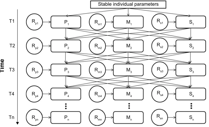
which health is seen in a systemic way, with mutual interac-tions among components. This means that each of the health components and the stable individual parameters may affect each other (Figure 1).

In addition to the above specifics, and in order to define the conceptual model as a dynamic systems model, the following characteristics are relevant: 1) the role of time, assuming that HRQOL is a construct that can develop in time; 2) the nonlinearity, assuming that the relations among components may be nonlinear with the possibility of drastic changes, reductions, or resource limitations.

Figure 1 represents the dynamic systems conceptual model of HRQOL. In particular, the upper box represents the stable individual parameters, including age, presence of diseases, and health behaviors (protective and risk fac-tors). The central part of the model is composed of the three health domains. Since the HRQOL model aims to represent longitudinal trends, each domain is connected with itself in a subsequent time point. Furthermore, the systemic approach is represented by the connections between each domain and the other two. Finally, each of the three domains of health is connected with a random influence, representing the unpre-dictable life events that may occur in any time point. In the

(4)

Dovepress

roppolo et al

figure, we represent only the first four iterations. However, the process and thus the series of iterations continue until a generic end point (Tn).

Material and methods

Mathematical translation of the

conceptual model

Translation procedure

In order to translate the model presented in Figure 1 into a mathematical model, it was necessary to replace arrows with equations. The translation procedure implies that all variables and relations need to be quantified. Measurements of HRQOL components are represented in a continuum between two extreme points, seen as the lowest and highest possible func-tions and percepfunc-tions in each health domain. It was chosen as an arbitrary scale of continuous values between 0 (worst HRQOL condition) and 1 (best HRQOL condition) for all components. Note that the choice of the scale is arbitrary and that the numbers have no intrinsic meaning, but only meaning in relation to each other. The only exceptional range is those of the random influences that vary between -1 (worst possible random influence) and 1 (best possible influence). Theoretically and intuitively, this implies that chance events can enhance, maintain stability, or reduce each HRQOL component.

The development of the system and its components is iterative, as expressed in Figure 1. Each iteration produces an outcome, which is generated by the quantitative relationships

expressed in equations. This outcome serves as input in the next iteration.24,29_{Depending on one’s research interests, the}

system can simulate few iterations, or a long range of itera-tions, representing a long period of time. From a dynamic systems point of view, the iterations should be frequent enough to reproduce a trajectory of change on a particular timescale, which in this particular case is the timescale of change over months or years.

The HRQOL quantitative model consists of one equation for each grower, and thus for each health domain (expressed as the average level between the self-report health status and experienced-health components). The equations specify how the grower changes as a function of itself and the other components in the system in each iteration. Specifically, each health domain grower is a function of the values of 1) itself, 2) other growers inside the system, 3) stable indi-vidual parameters, 4) random influences, and 5) additional parameters.

The mathematical model presented here is a nonlinear model of connected growers based on dynamic systems theory. Previous studies have built this type of model starting from the dynamic growth theory and the dynamic growth models.23,24,29–31_{The basic equation that supports}

these models is the logistic growth equation.22,24_This

equa-tion is particularly suitable in the analysis of living systems development, due to its nonlinear trend and maximum growth capacity; typical characteristics in human and psychological

6WDEOHLQGLYLGXDOSDUDPHWHUV

7LPH

5S

7 5P 5V

5V

5VQ 5P

5P

5PQ

3 0 6

6

6Q 0

0

0Q 3

3

3Q 5S

7

7Q

5S

5SQ

Figure 1 The conceptual dynamic systems model of hrQOl showing the interactions between the physical, mental, and social domains over time (T1 … Tn).

Notes: Stable individual parameters are an indicator of age, comorbidity, and lifestyle, directly influencing the three main domains of HRQOL; The model shows four iterations (from T1 to T4, and it shows how the process continues until a generic Tn), each arrow is a connection between domains during time, representing the influences of one factor on another, causing the influenced factor to change over time (dynamic relationship).

Abbreviations: hrQOl, health-related quality of life; P, physical domain; M, mental domain; s, social domain; rp, random factor in the physical domain; rm, random factor

in the mental domain; rs, random factor in the social domain.

(5)

sciences.32,33_{The logistic growth model will also serve as the}

basis for our model of HRQOL development.

Each equation needs some numerical input, in particular: 1) an initial value, 2) a growth rate, and 3) the level of growth capacity. The basic form of the logistic growth equation is the following equation:

L L L r rL

K

t

t t t

+ =

+ −

1

2

( )

(1)

where: 1) L_t is the value of the grower at a certain time t (at the first iteration it is the initial value); 2) r is the growth rate for each grower; and 3) K is the growth capacity.

The model was created and written on a Microsoft Office Excel spreadsheet.

Description of the equations

The three domains of HRQOL (physical, mental, and social) are each quantified by a logistic growth equation. Intersubject differences are represented in a set of parameters. This set is composed of 1) stable individual parameters, assumed as age, presence of diseases, and health behaviors; 2) a change rate for the stable individual parameters for each grower, due to the different effect that the development of the stable indi-vidual parameters may have on the three main components; 3) initial value for each grower, since it is necessary to enter a starting point in order to run a simulation. The starting point can be chosen by the researcher, in which case, the simulation is purely theoretical; otherwise, if the aim is to simulate the development of an individual, the initial value derives from empirical measurements; 4) growth rate for each grower; 5) adaptability to internal–external influences, intended as the individual ability to cope with and react to stressful life events, avoiding negative impact on health status and func-tions. The connection between the three domains (or growers) is realized by including in the equation for each grower the value of both other growers.

The development over time of the model is described in the series of iterations. In this model, each iteration represents 1 day, because it is assumed that 1 day is a kind of unit, and that the next day can be seen as a next unit. A daily time level represents a useful unit of experience. Daily data of HRQOL may be useful to detect developmental trajectories and patterns of changes that may serve as early indicators of negative health outcomes.

In each iteration, the growers’ equations are influenced by their own previous value, their growth rate, the para meters, the rate of changes of the other growers, and a random number representing the chance-related influence. All these

components play a role in the process of changes of HRQOL. The model is a continuous model in which each iteration represents a data point in a developmental path.

The model starts with the initial value for each grower. The following iteration is a function of the previous level of the grower and the growth rate.

L_t₊1= +L_t R_Lt (2)

The general growth rate (R_Lt) depends on the previous level of the grower, a composite growth rate, and the growth capacity.

R L r L

K

Lt t Lt

t

= × × −



 

 

1

(3)

The composite growth index is a function of the increase part of the equation and the chance value.

r_Lt =I_Lt ×C_Lt (4)

The chance component is the difference between two randomly selected numbers from 0 to 1. This technical solu-tion was adopted to guarantee randomizasolu-tion in the chance component of the model.

C_Lt =Random

[ ]

0 1− −Random

[ ]

0 1− (5)

This results in the generation of a random number in the range between -1 and +1, in which the chance that a num-ber around 0 is generated is higher than the chance that an extreme value (close to -1 or +1) is generated. This number, computed for each iteration, may be a good representation of daily unpredictable events that are very often small (close to zero), while bigger life events (with a value close to +1 or -1) are less common.

Finally, the increase part depends on the adaptability parameter, the growth rate of the other growers, and its growth rate parameter.

I_Lt A RMt RNt G

L

= ×

{

+

}



 



  +

2 (6)

where: 1) L_t is the value of the grower at a certain time t; 2) R is the general growth rate for each iteration; 3) r is the composite growth index; 4) K is the growth capacity, representing the limitations of resources; 5) I is the increase rate; 6) C is the random part of the model; 7) A is the adapt-ability parameter; 8) R_M and R_N are the growth rates of other growers (called here M and N); in the first iteration the initial

(6)

Dovepress

roppolo et al

condition parameter is used in place of R_M and R_N; 9) G is the growth parameter.

The equation is computed for each iteration in each grower. If the model is run for several cycles, it produces a set of points (one for each iteration) that make up develop-mental trajectories of the three components.

First procedure to test the validity of the

model

Before proceeding with an empirical validation analysis, the model was tested with a hybrid procedure. This procedure is called “hybrid” because it combines theoretical assumptions and numerical trajectories.22_{This procedure (defined}

cali-bration) aims to estimate the theoretical adherence of simu-lated data starting from sets of numerical data. The scopes of this analysis are 1) to test if the simulated trajectories, produced by the model, are theoretically plausible, starting from a given set of initial and parameter values; 2) to iden-tify within which ranges the parameters generate realistic trajectories (that do not get stuck to zero or explode into infinity). For all models, the range of parameter values is selected in such a way that a more or less realistic trajectory will result out of them. In other words, outside that range, the model may explode to infinity or get stuck at zero.

Several different sets of initial and parameter values, selected on theoretical possibilities, were simulated and analyzed in order to calibrate the model. For simplicity, just a selection of these patterns is reported here. Each pattern was run 200 times and qualitative results about developmental trends were collected.

set 1

The first set of initial and parameter data refers to normal conditions of life, and so normal starting values. It is to notice that normal is intended as a common and more or less average situation in real life. Three different patterns of starting data were used. The choice was arbitrary, with a selection of different combination of values. High and low values were defined on the basis of predefined range (0–1). Values seemed plausible, on a theoretical basis, in their combination, and covered a big part of the predefined range. These patterns represent different types of people. In particular, the first hypothetical person depicted here is related to an older adult (named “X”) who has some physical impairments. These physical problems limit his ability to walk autonomously inside and outside his home, making his HRQOL poor in all of the three domains. For this reason, the initial levels of the growers are set at 0.20. Since the

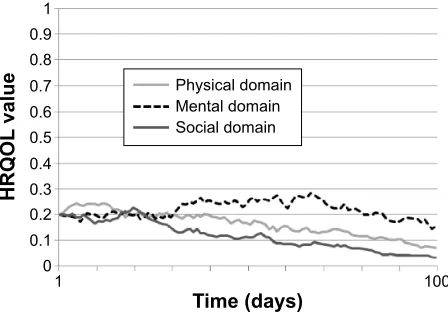
physical impairment is of a chronic nature, it is expected that the health conditions will decrease; so the growth rates for each domain are negative (-0.20). Despite the poor health condition (eg, presence of a chronic disease), “X” is relatively young (eg, 67-year-old) and so with a midlevel of the stable individual parameter that is set at 0.50. Fur-thermore, “X” continues to have a fairly good adaptability to stressing events; this is the reason why the adaptability parameter is set at 0.80. The developmental trajectory of “X” is presented in Figure 2.

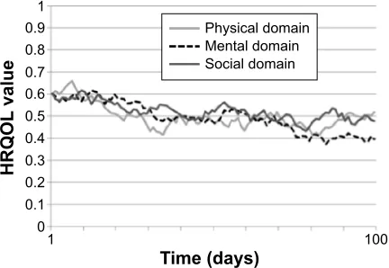
The second hypothetical older adult (called “Y”) has a better, but not optimal, health condition. The initial level for each domain is set at 0.40. Furthermore, his health is increas-ing, because he was engaged in a physical training class in the last month. This new habit allows “Y” to develop a bet-ter physical and mental health status, in association with an increase in his social activities. For these reasons, the growth rates are all set at 0.20. The stable individual parameters (due to age and presence of diseases) are medium (0.60) as well as the adaptability parameter (0.60). The developmental trajectory of “Y” is presented in Figure 3.

The third hypothetical subject (called “Z”) is a healthy and “young” older adult, with a medium to high initial levels for each domain (0.60). Unfortunately, due to the death of a relative, the general condition of “Z” is decreasing, with negative growth rates in each domain (-0.20). However, the stable individual parameters, due to young age (eg, 65 years) and absence of diseases are good (parameter set at 0.70). Finally, “Z” continues to cope fairly well with life events,

7LPHGD\V

+542/

YDOXH

3K\VLFDOGRPDLQ 0HQWDOGRPDLQ 6RFLDOGRPDLQ

Figure 2 hrQOl developmental trajectory of subject X with low initial values in

all domains.

Notes: Time (X-axis) is represented by means of the number of iterations computed by the model, assuming that one iteration represents 1 day; the Y-axis represents the level of hrQOl on a scale ranging from 0 to 1; in this particular simulation, the mental domain shows a slight increase, followed by a later decline whereas the physical and social domains start to decline relatively early.

Abbreviation: hrQOl, health-related quality of life.

(7)

with an adaptability parameter set at 0.80. The developmental trajectory of “Z” is presented in Figure 4.

The results of the simulated trajectories of “X”, “Y”, and “Z” are reported in Table 1 (first three rows). The first eight columns of the table report the patterns of data that were used to simulate trajectories. The following columns represent the behavior of the simulations, expressed in per-centages. It was tested whether the simulations exploded or get stuck to 0, whether they showed an increase or a decrease as compared to the initial situation, and a qualitative estima-tion of the theoretical plausibility of the trajectory assigned by the authors.

Information about the distribution of outcomes derived by specific sets of initial and parameter values is useful to get an impression of the plausibility of model’s behavior.

In particular, it was hypothesized that the majority of cases in the trajectories of first and third sets of initial and parameter data would produce lower final results in compari-son with the baseline data, because of their negative growth rates. This assumption is found to be true approximately 80% of times (Table 1). The remaining 20% of cases explain that, during the iterations, connections among variables and random fluctuations produced higher final results. This condition is compliant with reality, because it is possible to observe in real life that negative individual parameters (eg, an accident) not always develop in negative outcomes. A similar reasoning was made for the second condition: this represents a rather positive situation, and we expected and found overall positive development.

Finally, it is important to notice that all conditions pro-duced dynamic trends, with fluctuations and sudden jumps, and without completely rigid or exploded trajectories.

set 2

The second set of initial and parameter data refers to particu-lar conditions in which positive or negative accidental life events, occur, or in which the starting point may be unusual. For example, a physical healthy subject has an accident caus-ing a negative physical change rate. On a theoretical basis, we would expect that in such cases the physical domain often shows a decreasing trend, which can afflict also other domains.

On the contrary, a depressed older adult may meet an old friend, which may help him to be more satisfied about his life. It is conceivable that mental domain may have an increasing trend most of the time, influencing positively also other domains.

Finally, it is also possible to hypothesize subjects with mixed situations, in which a high social starting point is associated with a low change rate and vice versa for the psychological domain etc. These are just some examples, but they can represent real situations. For this reason, it is important to test the model’s behavior for such hypothetical subjects as well. Also in this case, we used three different conditions to calibrate the model. In summary, we ran simu-lations with six different sets of initial and parameter data: the first three represent nonoptimal, moderately optimal, and optimal initial conditions, respectively, and the last three represent a combination of optimal and nonoptimal conditions. For each set, we assessed how often the model

7LPHGD\V

+542/

YDOXH

Figure 3 hrQOl developmental trajectory of subject Y with moderate initial

values in all three domains.

Notes: Time (X-axis) is represented by means of the number of iterations computed by the model, assuming that one iteration represents 1 day; the Y-axis represents the level of hrQOl on a scale ranging from 0 to 1; in this simulation, all the three

domains show an increasing trend. The mental domain has more fluctuations than

the other two, whereas the social domain presented the highest increase.

7LPHGD\V

+542/

YDOXH

Figure 4 hrQOl developmental trajectory of the healthy and young subject Z with

high initial values in all domains.

Notes: Time (X-axis) is represented by means of the number of iterations computed by the model, assuming that one iteration represents 1 day; the Y-axis represents the level of hrQOl on a scale ranging from 0 to 1; all the domains show a decreasing

trend, more evident in the first iterations. In the final iterations, physical and social

domains show an increase, whereas the mental domain remains more stable.

(8)

Dovepress

roppolo et al

generated a completely static trajectory (assumed to be less plausible) and how often the simulation exploded to infinity (assumed to be impossible). In addition, we assessed how often the simulation showed the increase or decrease over time that was assumed to be most plausible on a theoretical basis. The results are shown in Table 1.

Within a wide range of initial and parameter values, the model generates theoretically plausible trends, because no stable or exploding trajectories were seen and, in addition, theoretical expectations (related to the mix of initial values and growth rates of the three domains) were generally confirmed.

The qualitative results proposed in Table 1 support the goodness of the model, but it is important to notice and to take into account for further analysis that the model does not work with some so-called “dangerous initial and parameter data.” These data are patterns of values that make the trajectories completely stable or completely random. In particular, very low change rates (lower than 0.02) in the three growers, in association with a low adaptability parameter (lower than 0.40) produce very stable (with very low fluctuations during the whole trajectory) and unchangeable developmental trajecto-ries. In addition to this, low levels of initial values in the three growers seem to increase the stability (Figure 5). Values pro-ducing such low-level rigid trajectories can be hypothesized to form the lower limits of the plausible data range.

On the contrary, higher change rates (higher than 0.80) in association with high values of the adaptability parameter (higher than 0.80) and with the increase of the grower’s ini-tial values bring trajectories to the maximum capacity level, after a first phase of dynamic trends (Figure 6). The values generating such extreme high-level trajectories could be seen as the upper limits of the usable data range.

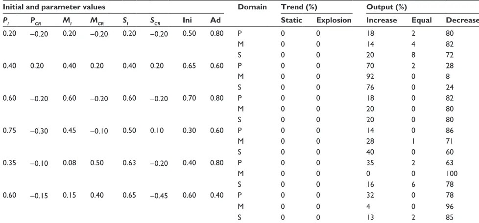
Furthermore, the change rates for the stable individual parameters were always set between -0.1 and 0.1. These Table 1 Qualitative outcomes of the calibration procedure, analyzing trends and final results of simulated data starting from different

sets of initial and parameter values

Initial and parameter values Domain Trend (%) Output (%)

PI PCR MI MCR SI SCR Ini Ad Static Explosion Increase Equal Decrease

0.20 -0.20 0.20 -0.20 0.20 -0.20 0.50 0.80 P 0 0 18 2 80

M 0 0 14 4 82

s 0 0 20 8 72

0.40 0.20 0.40 0.20 0.40 0.20 0.65 0.60 P 0 0 70 2 28

M 0 0 92 0 8

s 0 0 76 0 24

0.60 -0.20 0.60 -0.20 0.60 -0.20 0.70 0.80 P 0 0 18 0 82

M 0 0 20 0 80

s 0 0 20 0 80

0.75 -0.30 0.45 -0.10 0.50 0.10 0.30 0.60 P 0 0 14 0 86

M 0 0 28 1 71

s 0 0 40 0 60

0.35 -0.10 0.08 0.50 0.63 -0.20 0.40 0.80 P 0 0 35 2 63

M 0 0 0 0 100

s 0 0 16 6 78

0.60 -0.15 0.15 0.40 0.65 -0.45 0.60 0.40 P 0 0 32 0 78

M 0 0 4 0 96

s 0 0 13 2 85

Abbreviations: P, physical domain; M, mental domain; s, social domain; PI, initial value of the physical domain; PCR, change rate of the physical domain; MI, initial value

of the mental domain; MCR, change rate of the mental domain; SI, initial value of the social domain; SCR, change rate of the social domain; Ini, stable individual parameters;

Ad, adaptability parameter.

7LPHGD\V

+542/

YDOXH

Figure 5 extremely low developmental trajectory.

Notes: Time (X-axis) is represented by means of the number of iterations computed by the model, assuming that one iteration represents one day; the Y-axis represents the level of hrQOl on a scale ranging from 0 to 1; with this set of parameters and initial data all the domains remain stable for the entire period showing very subtle

fluctuations.

(9)

parameters allow to compute the role and the impact of changes in individual conditions on the three growers dur-ing time.

Validation procedure

The first empirical validation procedure is a minimal require-ment that is needed to assume the model resemble empirical data in a satisfactory way.24_{It is possible to perform an initial}

validation with two data points, an initial value and a value after a period that is long enough to produce considerable change (for example).24,34_{The use of two waves of}

assess-ments is very limited for the validation of a dynamic systems model, because between the initial and final data points there is a long sequence of changes that are generated by the model, but not documented by empirical data. However, the aim of this analysis is to understand whether a theoretically based dynamic systems model of HRQOL is capable to predict the outcomes, based on a set of initial and parameter values, on the basis of a model of realistic mechanisms of change, to con-nect at least two time points. Once this objective is reached, it will be possible to proceed with further and more powerful validation analyses, with the use of time-serial data.

Empirical baseline values were used as initial data in the model. The model was run for a given number of iterations (ie, the number of days between the assessments). The pro-cedure generated simulated final values that can be compared with the empirical ones, in order to analyze the empirical representativeness of the model. In other words, a known initial condition was entered in the model. The trajectories simulated by the model were compared with the empirical ones (based on real data).

Participants

Data used in the validation procedure derived from a sample of older adults (over 65 years) involved in an Italian Regional project, called ACT ON AGING, funded by Regione Piemonte. A total of 367 community dwelling older adults was involved.

The following inclusion criteria have been set: 1) age over 65 years, 2) Mini-Mental State Examination (MMSE) score higher than 25 (indicating absence of cognitive impairments), 3) independence in the activities of daily living, 4) ability to walk 500 m without assistance. While the exclusion criteria were 1) myocardial infarction and/or coronary bypass sur-gery in the last year, 2) uncontrolled diabetes or hyperten-sion, 3) orthopedic impairment and/or limbs fracture within the last 6 months, 4) simultaneous participation in another study. These criteria were chosen in order to have a sample of autonomous and quite healthy participants, with the pos-sibility to participate in an intervention study design.

Baseline and post test data of 194 subjects have been used in this study. Subjects who missed at least one question were excluded from the analysis. This method was preferred instead of a replacement method, because using only real data increases the reliability of the outcomes. The price paid for greater reliability was the reduction of the sample size. However, a total sample of 194 individuals was sufficient for the validation procedure.

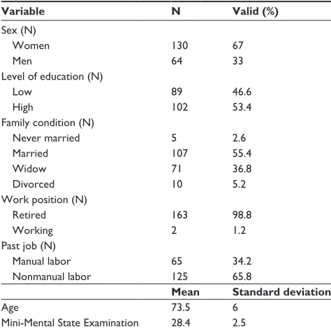
The whole sample was slightly unbalanced in terms of sex composition. The majority of participants were women (n=130; 67%). However, this composition reflects the Italian sex distribution among older adults. In fact, demographic data state that, in Italy, the number of aged (over 65) women is higher than the number of men.35

The mean age of the participants was 73.5 years (range: 65–90) and their score of MMSE was comprised between 25.2 and 30.0. All the participants were independent and noninstitutionalized.

The Ethical Committee of the University of Torino approved the study. All the participants were informed about the voluntary and confidential participation in the study. All the selected individuals gave their written informed consent in accordance with Italian law and the ethical code of the American Psychological Association.36

The descriptive characteristics of the participants are presented in Table 2.

research protocol

The general aim of ACT ON AGING was to determine the effectiveness of both physical and cognitive interventions on

7LPHGD\V

+542/

YDOXH 3K\VLFDOGRPDLQ

0HQWDOGRPDLQ 6RFLDOGRPDLQ

Figure 6 extremely high developmental trajectory.

Notes: Time (X-axis) is represented by means of the number of iterations computed by the model, assuming that one iteration represents 1 day; the Y-axis represents the level of hrQOl on a scale ranging from 0 to 1; with this set of parameters and initial data all the domains rapidly increase to the maximum values and then remain stable.

(10)

Dovepress

roppolo et al

the health status of participants. After the baseline assess-ment, the whole sample was split into three subgroups: two experimental groups that took part in physical or cognitive intervention and one control group. The experimental groups performed 16 weeks of activities, two sessions per week. The control group did not change its habits while performed only the evaluation trials. Measures were collected before and after the interventions on the whole sample.

For this study, the initial aim was to simulate HRQOL trajectories for each subgroup separately. However, no dif-ferences in HRQOL scores were found between initial and final data in each group. For this reason, it was decided not to consider the experimental allocation for each subject. Instead, the groups were differentiated by performing a cluster analysis in order to split the sample in groups with different starting values and change rates in time.

Measures

The physical, mental, and social components of HRQOL were collected with validated self-report questionnaires.

The Short Form 36 Health Survey (SF-36;37_{), the Lubben}

Social Network Scale-6 (LSNS-6;38_{), and the Friendship}

Qual-ity Scale (FQS;39_{) were used to assess the three components}

of HRQOL delineated in the conceptual model. Specifically, the physical domain was rated with the SF-36 physical health summary measure (PCS), the mental domain was assessed with the SF-36 mental health summary measure (MCS), and the social domain was measured with the LSNS-6 and the FQS.

The SF-36 is one of the most used instruments to assess health status and HRQOL.18_{The SF-36 is composed of two}

summary measures (PCS, composed of 21 items; MCS, composed of 14 items). The use of the SF-36 in the aged population is well documented in previous research.40–44

The LSNS-6 is a six-item scale that is widely used to assess social network in aged persons.38,45_{The LSNS-6 is}

specifically designed for older adults, and it is useful for measuring their social isolation.

Finally, the FQS is an instrument specifically designed for aged population that measures social isolation and quality of social relationships.39,46

Both LSNS-6 and FQS questionnaires were chosen to assess the social domain for the following reasons: 1) the social domain is a crucial component of HRQOL, especially in an older adult population. Furthermore, many aspects need to be taken into account, in order to have a view of the social domain that is as complete as possible. For these reasons, it was decided to use both scales. 2) The two scales used to mea-sure the social sphere capture different aspects of the domain. In particular, the LSNS-6 questions are more self-report health status oriented, asking the number of persons attended in the last month. The FQS tends to capture more experienced-health about social life. As expressed in our theoretical model, and in accordance with Kelley-Gillespie,47_{the simultaneous use of}

these two measures allows us to analyze both dimensions. All the instruments are self-report; however, a psy-chologist was present during the initial and final assessments to give support in case of doubts or difficulties in the questionnaires’ completion (ie, difficulty to read questions or to understand their meaning).

Data from the two waves were transformed in order to 1) give them the same directions, and 2) make them compa-rable with the simulated data produced by the model. Since the simulated data ranged between 0 and 1, the following formula was used to transform the empirical data to the same scale:

y= x− −

M

M M

in

ax in (7)

where, y is the output of the transformation (a number varying from 0 to 1 on a continuous scale); x is the empirical data; min is the minimum value of the scale, and max is the maximum value of the measure. This transformation maintains the original distribution characteristics, allowing an easy good comparison between simulated and empirical data.

To test the indexes reliability, a Cronbach’s α analysis was performed. All the domains in both initial and final assessments were found to have a satisfactory internal Table 2 Baseline characteristics of the participants

Variable N Valid (%)

sex (n)

Women 130 67

Men 64 33

level of education (n)

low 89 46.6

high 102 53.4

Family condition (n)

never married 5 2.6

Married 107 55.4

Widow 71 36.8

Divorced 10 5.2

Work position (n)

retired 163 98.8

Working 2 1.2

Past job (n)

Manual labor 65 34.2

nonmanual labor 125 65.8

Mean Standard deviation

Age 73.5 6

Mini-Mental state examination 28.4 2.5

(11)

consistency, with an α level always higher than 0.70 (Table 3).48_{For these reasons, it was decided to use a single}

index of social domain aggregating the scores of LSNS-6 and FQS questionnaires.

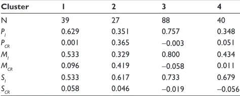
Finally, a hierarchical and a K-means cluster analysis was performed, combining baseline and change rate values (final – baseline data), in order, first, to understand in how many subgroups the whole sample can be split and, second, to set and compute central values for each cluster. The best solution turned out to be a four-cluster solution. The cluster centers are reported in Table 4.

statistical analyses

The starting values used to run the model were the empirical clusters data. In addition to the growers values (initial value and change rate), a set of parameters must be set.

To determine the value for the parameter called stable individual parameters we created an index based on the age of participants and the presence of diseases. For the grow-ers, the parameter value is located on a continuous scale ranging between 0 and 1, where 1 is the best possible score (ie, 65 years and without diseases). The cluster values for this parameter were Cluster 1, 0.530; Cluster 2, 0.547; Cluster 3, 0.557; Cluster 4, 0.563.

The adaptability parameter was always set at 0.80, due to the generally good health conditions of the sample. The change rates for the stable individual parameters were set between -0.1 and 0.1. This range was chosen for theoretical reasons and after the good results achieved in the calibration procedure. The growth capacity was set at 1.0.

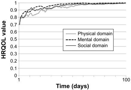
Once that the values of the parameters and the initial conditions have been chosen, it is possible to run the model. With this procedure, the model simulates data for the num-bers of iterations requested. In this study, it was used 100 iterations. Each iteration represents a day. In this way, it was simulated a number of days that is similar to the time between baseline and final measurement in the empirical sample. The values for each grower (P, M, and S) at T100 represent the simulated final data.

A three-step statistical analysis was performed to compare the empirical and the simulated outcomes for the validation of the model. First, a Monte Carlo simulation test was used to analyze differences between the empirical and simulated final data for each cluster group. Second, the final empirical and simulated distributions were compared using nonparametric test (Wilcoxon test), in order to analyze differences among the results. Third, a series Kruskal–Wallis test in addition to Mann– Whitney U- test post hoc with the use of Dunn-Sidak correction, was performed in order to analyze the correspondence among statistical differences (among clusters) in 1) empirical vs empir-ical, 2) simulated vs simulated, and 3) simulated vs empirical data. In other words, these tests allowed to know whether the prediction made with the model reflects real data.

While the first two steps aim to analyze similarities between simulated and empirical results in the same cluster, the third procedure aims to highlight correspondences in the differences among different clusters.

The Monte Carlo simulation technique was used to test differences between the output values produced by the model and the empirical final data. An in-depth explanation about the Monte Carlo technique was published by Kunnen.22

Specifically, this method generates a given number (1,000 in this case) of simulated final data, comparing these results with the empirical ones. During the procedure, the number of times that simulated data are higher or lower than empirical ones is computed, giving an associated P level, to understand the probability that the differences between the model and the data could be explained on the basis of chance while in fact, the empirical and simulated data are both part of the same set of data. The best fit is represented by a level of P near 0.50, meaning that the model produces for 50% of times higher simulated data and the other 50% of times lower simulated data in respect to the empirical ones. For this reason, a level of P which deviates much from 0.50 (eg, P=0.70) becomes unacceptable. Three Monte Carlo procedures were carried out for each cluster. This was done in order to test whether the selected range for the change rate of the stable individual parameters was acceptable. First, the Monte Carlo technique Table 3 Cronbach’s α analysis of indexes

Wave 1 n

P 0.862 0.876

M 0.870 0.873

s 0.797 0.756

Abbreviations: Wave 1, baseline assessment; Wave n, final assessment; P, physical

index; M, mental index; s, social index.

Table 4 Cluster centers

Cluster 1 2 3 4

n 39 27 88 40

P_I 0.629 0.351 0.757 0.348

P_CR 0.001 0.365 -0.003 0.051

MI 0.533 0.329 0.800 0.434

M_CR 0.096 0.419 -0.058 0.011

SI 0.533 0.617 0.733 0.679

S_CR 0.058 0.046 -0.019 -0.056

Abbreviations: PI, initial value of the physical domain; PCR, change rate of the

physical domain; MI, initial value of the mental domain; MCR, change rate of the mental

domain; SI, initial value of the social domain; SCR, change rate of the social domain.

(12)

Dovepress

roppolo et al

was run using the extreme data range (-0.1 and 0.1) in each grower. Second, for the definitive analyses we used the change rate values of the stable individual parameters that resulted in the best fit.

Moreover, a comparison between simulated and mea-sured final results was given with a nonparametric test for dependent sample (Wilcoxon test). The Wilcoxon test was chosen for the nonnormality of data, for the low clusters sample size (min =20; max =88). The final data produced by the model consisted of 1000 simulated outcomes. A random subsample of simulated outcomes with the same size of the empirical sample was extracted with a shuffle technique (that allows to extract cases from the simulated distributions without replacement). This was done, because a large sample of empirical data would increase the chance of significant findings. Finally, the Wilcoxon test between the two distributions was performed, in order to highlight the statistically significant differences. The optimal outcome in terms of validity of the model is represented by the absence of statistically significance differences among the distributions, meaning that a subsample of data produced by the model is not different from the empirical data.

A series of Kruskal–Wallis tests was computed in order to analyze differences among clusters. This analysis was performed to compare different empirical clusters, different simulated clusters, and simulated with empirical clusters. If the Kruskal–Wallis test shows that the difference among the clusters is statistically significant, a series of Mann–Whitney

U-tests with Dunn-Sidak corrections was performed to test the pairwise significance level. This step was necessary to test whether the model generates clusters that differ from each other in the same way as the empirical data. The best outcome is to find good resemblance among clusters in the empirical, simulated, and empirical vs simulated datasets.

Results

Simulated vs empirical final data

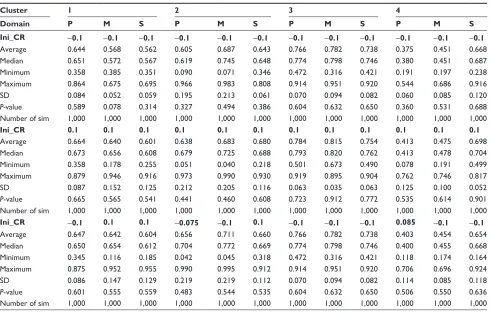
Monte Carlo test was used to compare 1,000 simulated data with the empirical final data. We compared simulated and empirical datasets with the same sets of stable parameters. The results of the Monte Carlo procedure are reported in Table 5.

In general, no differences were found in any of the compari-sons among domains and all clusters. The final data produced by the model resemble the empirical ones. The selected range for

Table 5 Monte Carlo analysis of the compared empirical and simulated outcomes, for different sets of initial change rates for each of the domains P, M, and s, and for the four different clusters

Cluster 1 2 3 4

Domain P M S P M S P M S P M S

Ini_CR -0.1 -0.1 -0.1 -0.1 -0.1 -0.1 -0.1 -0.1 -0.1 -0.1 -0.1 -0.1

Average 0.644 0.568 0.562 0.605 0.687 0.643 0.766 0.782 0.738 0.375 0.451 0.668

Median 0.651 0.572 0.567 0.619 0.745 0.648 0.774 0.798 0.746 0.380 0.451 0.687

Minimum 0.358 0.385 0.351 0.090 0.071 0.346 0.472 0.316 0.421 0.191 0.197 0.238

Maximum 0.864 0.675 0.695 0.966 0.983 0.808 0.914 0.951 0.920 0.544 0.686 0.916

sD 0.084 0.052 0.059 0.195 0.213 0.061 0.070 0.094 0.082 0.060 0.085 0.120

P-value 0.589 0.078 0.314 0.327 0.494 0.386 0.604 0.632 0.650 0.360 0.531 0.688

number of sim 1,000 1,000 1,000 1,000 1,000 1,000 1,000 1,000 1,000 1,000 1,000 1,000

Ini_CR 0.1 0.1 0.1 0.1 0.1 0.1 0.1 0.1 0.1 0.1 0.1 0.1

Average 0.664 0.640 0.601 0.638 0.683 0.680 0.784 0.815 0.754 0.413 0.475 0.698

Median 0.673 0.656 0.608 0.679 0.725 0.688 0.793 0.820 0.762 0.413 0.478 0.704

Minimum 0.358 0.178 0.255 0.051 0.040 0.218 0.501 0.673 0.490 0.078 0.191 0.499

Maximum 0.879 0.946 0.916 0.973 0.990 0.930 0.919 0.895 0.904 0.762 0.746 0.817

sD 0.087 0.152 0.125 0.212 0.205 0.116 0.063 0.035 0.063 0.125 0.100 0.052

P-value 0.665 0.565 0.541 0.441 0.460 0.608 0.723 0.912 0.772 0.535 0.614 0.901

number of sim 1,000 1,000 1,000 1,000 1,000 1,000 1,000 1,000 1,000 1,000 1,000 1,000

Ini_CR -0.1 0.1 0.1 -0.075 -0.1 0.1 -0.1 -0.1 -0.1 0.085 -0.1 -0.1

Average 0.647 0.642 0.604 0.656 0.711 0.660 0.766 0.782 0.738 0.403 0.454 0.654

Median 0.650 0.654 0.612 0.704 0.772 0.669 0.774 0.798 0.746 0.400 0.455 0.668

Minimum 0.345 0.116 0.185 0.042 0.045 0.318 0.472 0.316 0.421 0.118 0.174 0.164

Maximum 0.875 0.952 0.955 0.990 0.995 0.912 0.914 0.951 0.920 0.706 0.696 0.924

sD 0.086 0.147 0.129 0.219 0.219 0.112 0.070 0.094 0.082 0.114 0.085 0.118

P-value 0.601 0.555 0.559 0.483 0.544 0.535 0.604 0.632 0.650 0.506 0.550 0.636

number of sim 1,000 1,000 1,000 1,000 1,000 1,000 1,000 1,000 1,000 1,000 1,000 1,000

Notes: Average, the average outcome of 1,000 simulations; minimum, the lowest outcome of the 1,000 simulations; maximum, the highest outcome of the 1,000 simulations;

P-value, chance that the empirical outcomes and the simulated outcomes stem from the same distribution of data.

(13)

the change rate of the stable individual parameters resulted in a good fit of the model with empirical data. In fact, no differences were detected in each pairwise comparison, both for the lower (-0.1) and for the higher (0.1) bound of the range. The values for the change rates were estimated, since it was not possible to assess this parameter. The values that created distributions that are closest to the empirical ones were chosen.

The average P-value level in the model is 0.57 (P=0.55;

M=0.57; S=0.59). This outcome shows that the distribution of the final measurement simulated data is in about 50% of the simulations higher than the average of the empirical data, and in about 50% lower than the empirical data.

The high similarity between empirical and simulated data is a first result for the validation procedure, giving important information about the representativeness of the model.

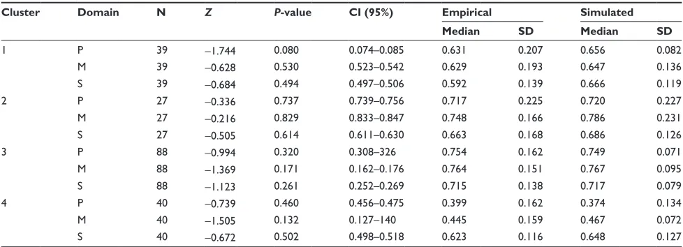
The second step in the validation analysis was the com-parison between simulated and empirical distributions with the same sample size. The results of the Wilcoxon test are shown in Table 6.

The absence of significant differences between the empirical and the simulated distributions indicates that the model faithfully reproduces reality. The results reported in Table 6 show that the P-value in each cluster and in each domain never achieves the level of significance set at 0.05 (min =0.080; max =0.829).

The simulated median values have an average dispersion rate of 3.68% (min =0.13%; max =12.69%) compared to the empirical ones. This information suggests that the simulated data are comparable with the real data.

Cross-comparisons among different domains

Once the similarities between the model and the real data were tested, it was necessary to investigate how the model

reacts to differences in stable individual parameters. As stated before, initial values affect the developmental outcome, and we want to test whether differences in initial values show the same differences in outcome in the empirical and in the simulated trajectories.

To test the effect of different initial values, the outcome distribution in each cluster was compared with 1) empirical outcome distributions of the other clusters, and 2) simulated outcome distributions of the other clusters. In order to provide an indication of the validity of the model, the empirical and the simulated outcome distributions should show similar differences in the same couples of clusters.

Simulated distributions were selected with a random extraction procedure.

The Kruskal–Wallis test reported significant differences in physical domain for empirical (H(3)=55.792, P,0.001), simulated (H(3)=96.381, P,0.001), and empirical vs simulated (H(3)=71.202, P,0.001) data. Similar results were found in mental domain for empirical (H(3)=62.596,

P,0.001), simulated (H(3)=88.170, P,0.001), and empiri-cal vs simulated (H(3)=70.200, P,0.001) data. Finally, the significant results in the social domain were for empirical (H(3)=14.171, P=0.003), simulated (H(3)=18.970, P,0.001), and empirical vs simulated (H(3)=13.924, P,0.001) data.

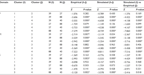
Since all the Kruskal–Wallis tests showed significant results, post hoc analysis with Mann–Whitney U-tests was conducted applying a Dunn-Sidak correction. The correc-tion resulted in a significance level set at P,0.008. Post hoc results are presented in Table 7.

The outcomes show strong resemblances both for the simu-lated and for the simusimu-lated vs empirical comparison in respect to the empirical results. Just in three cases (M domain cluster 1 vs cluster 2, simulated and empirical vs simulated; S domain

Table 6 Wilcoxon test for dependent samples, empirical vs simulated final data

Cluster Domain N Z P-value CI (95%) Empirical Simulated

Median SD Median SD

1 P 39 -1.744 0.080 0.074–0.085 0.631 0.207 0.656 0.082

M 39 -0.628 0.530 0.523–0.542 0.629 0.193 0.647 0.136

s 39 -0.684 0.494 0.497–0.506 0.592 0.139 0.666 0.119

2 P 27 -0.336 0.737 0.739–0.756 0.717 0.225 0.720 0.227

M 27 -0.216 0.829 0.833–0.847 0.748 0.166 0.786 0.231

s 27 -0.505 0.614 0.611–0.630 0.663 0.168 0.686 0.126

3 P 88 -0.994 0.320 0.308–326 0.754 0.162 0.749 0.071

M 88 -1.369 0.171 0.162–0.176 0.764 0.151 0.767 0.095

s 88 -1.123 0.261 0.252–0.269 0.715 0.138 0.717 0.079

4 P 40 -0.739 0.460 0.456–0.475 0.399 0.162 0.374 0.134

M 40 -1.505 0.132 0.127–140 0.445 0.159 0.467 0.072

s 40 -0.672 0.502 0.498–0.518 0.623 0.116 0.648 0.127

(14)

Dovepress

roppolo et al

cluster 3 vs cluster 4, simulated vs empirical data), we found a difference between empirical and simulated results, due to the fact that comparisons did not reach the P level of the Dunn-Sidak’s correction. In all the other cases, similarities were found among the three conditions.

Discussion

This work focused on the construction of a mathematical dynamic systems model of HRQOL. The goal of this dynamic systems model is to represent the theoretical mechanisms of the change of HRQOL over time, and not to represent a dataset. That means that the dynamic systems model is a mathematical formalization of the conceptual developmental model.19

A three-step procedure was followed to develop and validate the model: 1) first, the conceptual dynamic systems model was translated into a mathematical tool, replacing arrows with equations; 2) second, the new mathematical model was tested with a hybrid procedure (called calibration), in order to verify whether its simulated trends were theo-retically plausible; and 3) finally, the model was subjected to an initial empirical validation test based on the simplest possible empirical validity case, namely by connecting an initial measurement with a final measurement, separated by a duration that is long enough to correspond with consider-able change.

Table 7 Mann-Whitney U pairwise comparisons of simulated and empirical final data with Dunn-Sidak corrections

Domain Cluster (I) Cluster (J) N (I) N (J) Empirical (I–J) Simulated (I–J) Simulated (I) vs Empirical (J)

Z P-value Z P-value Z P-value

P 1 2 39 27 -1.076 0.282 -0.789 0.430 -1.376 0.169

1 3 39 88 -3.606 0.000* -6.058 0.000* -4.422 0.000*

1 4 39 40 -3.555 0.000* -6.658 0.000* -4.158 0.000*

2 3 27 88 -1.759 0.079 -1.149 0.136 -1.650 0.099

2 4 27 40 -3.733 0.000* -4.538 0.000* -4.167 0.000*

3 4 88 40 -7.279 0.000* -8.739 0.000* -7.860 0.000*

M 1 2 39 27 -2.719 0.007* -2.119 0.034 -2.367 0.018

1 3 39 88 -3.559 0.000* -5.545 0.000* -5.138 0.000*

1 4 39 40 -3.942 0.000* -5.354 0.000* -3.716 0.000*

2 3 27 88 -0.148 0.882 -0.046 0.963 -0.831 0.406

2 4 27 40 -5.369 0.000* -4.385 0.000* -5.458 0.000*

3 4 88 40 -7.323 0.000* -8.811 0.000* -7.516 0.000*

s 1 2 39 27 -1.369 0.163 -0.776 0.438 -1.337 0.181

1 3 39 88 -2.993 0.003* -5.533 0.000* -4.429 0.000*

1 4 39 40 -0.098 0.922 -0.157 0.875 -0.726 0.468

2 3 27 88 -0.670 0.503 -1.759 0.073 -1.537 0.124

2 4 27 40 -1.470 0.141 -0.793 0.428 -0.971 0.331

3 4 88 40 -3.120 0.002* -3.578 0.000* -2.416 0.018

Notes: *Significant after Dunn-Sidak correction. I and J refer to the number of the clusters analyzed.

Abbreviations: n, number of subjects in each cluster; P, physical domain; M, mental domain; s, social domain; Z, zeta score based on the Mann-Whitney U-test.

Results reported here are positive and encouraging with regard to the validity of the model. The model was found to produce theoretically acceptable developmental trends. Furthermore, the three-step validation procedure returned positive results: the generated trajectories behaved according to theoretical expectations.

The results obtained in the analyses give fundamental information at two different levels. The first level is purely theoretical. In fact, the adherence between real and simulated data is a first confirmation of the theoretical model underly-ing the mathematical model, and thus, that it makes sense to consider HRQOL in the aging population as a dynamic system. This confirmation may represent a milestone in the study of aging development, making room for a clearer idea about structures, ways and mechanisms of development of the construct under study. In particular, results reported here seem to confirm our theoretical assumptions that 1) the domains included in the conceptual model are connected and are influencing each other; 2) the developmental pro-cess is nonlinear; 3) the measures are dependent in time; 4) random influences are relevant aspects of the dynamics.19

Furthermore, the development of the mathematical tool gives a quantitative translation to the theoretical assump-tions, providing more information that is useful for further theoretical enhancement.22_{The second level is more closely}

related to practical applications. The mathematical dynamic