Predicting Microstructural Pattern Formation Using Stabilized Spectral Homogenization

(1)

spectral homogenization

Thesis by

Vidyasagar

In Partial Fulfillment of the Requirements for the Degree of

Doctor of Philosophy (Ph.D.) in Aeronautics

CALIFORNIA INSTITUTE OF TECHNOLOGY Pasadena, California

2019

(2)

ORCID: 0000-0003-0262-5429

(3)

ACKNOWLEDGEMENTS

I would like to express my strong heartfelt gratitude to my adviser, mentor, teacher, and friend Prof. Dennis M. Kochmann. It has been a very enlightening journey, from first encountering his work on material instabilities as a young undergraduate in London, to joining his group at Caltech, and then following him on a sojourn to Switzerland. This work would not have been possible without his brilliant ideas, patient responses, and understanding nature.

Next I would like to extend my appreciation to my thesis committee. I am extremely honored to have had meetings and discussions with Prof. Bhattacharya and Prof. Ortiz. Prof. Ravi always been there for support and encouragement, from the very first time I visited Caltech.

I would also like to express immense gratitude to the wonderful Mechanics and Materials family, who made my time at Caltech and ETH Zürich memorable. My seniors Neel Nadkarni, Ishan Tembhekar, Yingrui Chang, Stan Wojnar, and Alex Zelhofer passed on to me the knowledge and foundation upon which this work is built. My group members Abbas Tutcuoglu, Carlos Portela, Greg Phlipot, Wei-Lin Tan, Sid Kumar, Basti Krödel, Romik Khajehtourian, Claire Lestringant, Bastian Telgen, and Raphael Glaesener made every day I spent with them a bright one. Our administrative staff, Denise Ruiz in Pasadena, and Maria Trodella in Zürich, deserve special mentions for their unwavering patience, kindness and life advice.

My friends at Caltech have been crucial sources of strength throughout this journey. They gave me much needed motivation to spend time outside work – be it on weekend brunches, hiking trips, or Vegas adventures. I particularly thank Matt Leibowitz, Christophe Leclerc, Nelson Yanes, Cecilia Huertas, Will Schill, Kavya Sudhir, Jaeyun Moon, Danilo Kusanovic, Chandru Dhandapani, Joel Lawson, Louisa Avellar, Dingyi Sun, Trenton Kirchdoerfer and Serena Ferraro. I am also indebted to Laura Flower Kim and Daniel Yoder of the International Office at Caltech (ISP), who made life significantly easier. I thank Christine Ramirez and Profs. McKeon and Meiron for their help with the academic process at GALCIT.

(4)

ABSTRACT

Instability-induced patterns are ubiquitous in nature, from phase transformations and ferroelectric switching to spinodal decomposition and cellular organization. While the mathematical basis for pattern formation has been well-established, autonomous numerical prediction of complex pattern formation has remained an open challenge. This work aims to simulate realistic pattern evolution in material systems exhibiting non-(quasi)convex energy landscapes. These simulations are performed using fast Fourier spectral techniques, developed for high-resolution numerical homogenization. In a departure from previous efforts, compositions of standard FFT-based spectral techniques with finite-difference schemes are used to overcome ringing artifacts while adding grid-dependent implicit regularization.

The resulting spectral homogenization strategies are first validated using benchmark energy minimization examples involving non-convex energy landscapes. The first investigation involves the St. Venant-Kirchhoff model, and is followed by a novel phase transformation model and finally a finite-strain single-slip crystal plasticity model. In all these examples, numerical approximations of energy envelopes, computed through homogenization, are compared to laminate constructions and, where available, analytical quasiconvex hulls.

Subsequently, as an extension of single-slip plasticity, a finite-strain viscoplastic formulation for hexagonal-closed-packed magnesium is presented. Microscale intragranular inelastic behavior is captured through high-fidelity simulations, providing insight into the micromechanical deforma-tion and failure mechanisms in magnesium. Studies of numerical homogenizadeforma-tion in polycrystals, with varying numbers of grains and textures, are also performed to quantify convergence statistics for the macroscopic viscoplastic response.

(5)

PUBLISHED CONTENT AND CONTRIBUTIONS

Vidyasagar, A., Tan, W. L., Kochmann, D. M. 2017. Predicting the effective response of bulk polycrystalline ferroelectric ceramics via improved spectral phase field methods. Journal of the Mechanics and Physics of Solids 106, 113-151.

URL:https://doi.org/10.1016/j.jmps.2017.05.017

A. V. developed and implemented numerical schemes. W.-L. T. set up and performed ex-periments under supervision of D. M. K.

Vidyasagar, A., Tutcuoglu, A., Kochmann, D. M. 2018. Deformation patterning in finite-strain crystal plasticity by spectral homogenization with application to magnesium. Computer Meth-ods in Applied Mechanics and Engineering, 335, pp.584-609.

URL:https://doi.org/10.1016/j.cma.2018.03.003

A. V. and A. T. jointly developed the numerical methods under the guidance of D. M. K.

Vidyasagar, A., Krödel, S., Kochmann, D. M. 2018. Microstructural patterns with tunable mechan-ical anistropy obtained by simulating anisotropic spinodal decomposition. Proceedings of the Royal Society A: Mathematical, Physical and Engineering Sciences 474, 20180535.

URL:https://doi.org/10.1098/rspa.2018.0535

(6)

LIST OF ILLUSTRATIONS

Number Page

1.1 Multi-scale nature of patterns in a butterfly wing that lead to structural iridescence (Thomé et al., 2014). Reproduced with permission. . . . 1

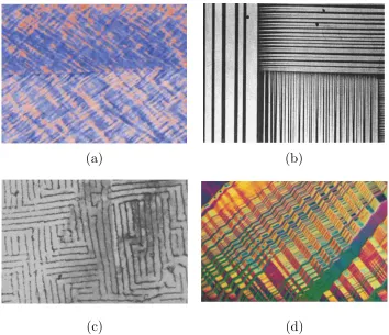
1.2 A series of natural patterns in mechanics that form from disordered initial states: (a) cross-hatched dislocation patterns in an Al bicrystal at the interface (Kuo et al., 2003), (b) twinning laminate structures in Cu-Ni (Abeyaratne et al., 1996), (c) labyrinth-type patterns in a fatigued Cu single crystal (Jin and Winter, 1984), (d) martensitic phase transformation domain patterns (Bhattacharya and James, 2005).

Reproduced with permission.. . . 2

1.3 Micrograph of striped domain patterns forming within grains of ferroelectric PZT polycrystal during fatigue cycling. Courtesy of Wei-Lin Tan, Caltech. . . . 3

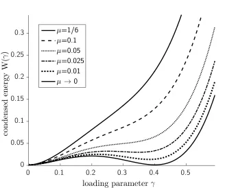
1.4 Loss of convexity of the condensed energyW(γ)with decreasing µ, forλ= 1. . . . 6 1.5 Examples of loss of convexity in systems exhibiting pattern formation.. . . 6 1.6 QW(F)for phase transitions withW(F)=min(W1(F),W2(F)). Spontaneous

break-down of the homogeneous blue and red phases at a deformation gradient state cor-responding to the quasiconvex envelope results in (non-unique) pattern formation. . 8 1.7 An overview of the variety of dislocation slip and twinning modes in magnesium. . . 12 2.1 An FFT-based interpolation of a rectangular function f(x) = rect(1₃,2₃) (a) results

in oscillatory approximations with the Gibbs phenomenon. Here, the slopes are shown in black at the grid points, and this directly results in the oscillations of the derivative f0(x), shown in(b), which is computed using the wave vector multiplied

by the Fourier transform of f(x).. . . 22 2.2 Spectral derivative of the double step function using first- and fourth-order

finite-difference correction, compared with classical FFT, and analytical solution (Vidyasagar et al., 2017). . . 26 2.3 Spectral derivative of the half-sine function using first- and fourth-order

finite-difference correction, compared with classical FFT, and analytical solution (Vidyasagar et al., 2017). . . 27 2.4 (a) Finite-difference approximation indicates loss of accuracy when the mesh

(9)

2.5 Stress distribution 11

µ_mat (a) the standard iterative spectral method (b) fourth-order finite-difference corrections and (c) first-order corrections (Vidyasagar et al., 2017). 28 3.1 Loss of convexity of the condensed energyW(γ)as the shear modulus µdecreases,

forλ= 1. . . 33 3.2 The calculated numerical hull shown in (a) shown near the origin in (b).

Corre-sponding microstructural patterns are shown in sequence in (c) during the loading process through the deformation gradient componentF₁₁. . . 34 3.3 The numerically calculated hulls atγ = −0.25 shown for different degrees of

non-convexity with given parametersλ=1 from (a) µ= 0.001 and (b)µ=0.01. . . 35 3.4 The largest patterns formed using first-order central difference approximation

demon-strate complexity of pattern formation, with each component of deformation showing different patterns that are compatible. . . 35 3.5 Plot ofF∗from (3.18) for the biaxial loading defined by (3.30) withµ=1 andκ =3

for various values ofkT from 0.001 to 0.05. . . 40

3.6 The calculated numerical hull is shown in (a). The corresponding microstructural patterns are shown in the volume fractions (b) & deformation gradient component F₁₂(c) during the loading process. . . 41 3.7 The calculated numerical hull is shown in (a) for the three-well case. The

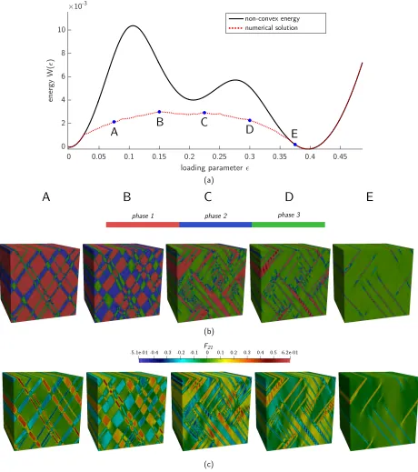
correspond-ing microstructural patterns are shown in the volume fractions (b) & deformation gradient component F₂₁ (c) during the loading process. . . 43 3.8 The calculated numerical hull is shown in (a) for the three-well case where the

ex-tremal wells lie below the middle-well. The corresponding microstructural patterns are shown in the volume fractions (b) & deformation gradient component F₂₁ (c) during the loading process. . . 44 3.9 Loss of convexity of the condensed energy A∗(λ) as the hardening parameter H

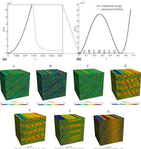
decreases (Vidyasagar et al., 2018). . . 46 3.10 Approximation of the quasiconvex envelope obtained by spectral homogenization

without finite-different approximation: the average energy of the RVE is compared to the non-convex condensed energy with (a) showing a magnification of (b); (c) shows the microstructural slip activity within the RVE at stages A through G along the loading path as indicated in (b) (Vidyasagar et al., 2018). . . 48 3.11 Approximation of the quasiconvex envelope obtained by spectral homogenization

(10)

3.12 Laminate patterns for the simple shear test case at λ = 0.208 obtained from (a) numerical simulations using the above spectral homogenization framework and (b) the equivalent sharp-interface description. (c) shows the local energy density dis-tribution of the numerical solution in (a), which shows concentrated energy within interfaces (Vidyasagar et al., 2018). . . 51 3.13 Influence of the slip system orientation ϕ on the non-convex, condensed energy

landscape of a single-crystal, with all shown energies exhibiting non-convexity at different range of values for the shear parameterλ(Vidyasagar et al., 2018). . . 53 3.14 Laminate pattern formation in bicrystals at an applied shear strain ofλ = 0.03: (a)

the geometric arrangement of the two grains within the bicrystal RVE along with the definition of angles ϕ₁and ϕ₂ in the blue and red grains, respectively. Results are shown for (b) ϕ₁ = −π/3 and ϕ₂ = −π/4, (c) ϕ₁ = −π/3 and ϕ₂ = −π/6, and (d) ϕ₁= −π/3 andϕ₂ =−π/12 (Vidyasagar et al., 2018). . . 54 4.1 An overview of the variety of dislocation slip and twinning modes in magnesium

(Vidyasagar et al., 2018). . . 61 4.2 (a) Effective stress-strain response of a simple shear test of an RVE containing 100

grains whose orientations are shown in the pole figure (b). (c) State of the RVE at an applied average shear strain ofF₁₂0 = λ=0.09. RVEs are shown in the deformed configuration, whereas the bounding box indicates the undeformed shape. Plots illustrate the grain shapes and components of the first Piola-Kirchhoff stress tensor

P as well as the distribution of prismatic slip and of the total volume fraction of

all extension-twinned regions. The shown stress distributions are in units of GPa (Vidyasagar et al., 2018). . . 64 4.3 Using the same grain geometry as in Fig. 4.2(a), an investigation is performed on how

the effective stress-strain response in (a) changes with increasing grain misorienta-tion, as shown by the pole figures in (b). Increasing the spread of the texture allows more easy-slip and -twin systems to become active across a larger number of grains, resulting in significant softening even at low strains. (c) The resulting shear stress distribution illustrates stronger stress differences and concentrations with increasing misorientation. The shown stress distributions are in units of GPa (Vidyasagar et al., 2018). . . 65 4.4 Polycrystalline case (E) of the simple shear experiment (see the pole figure in

(11)

4.5 Influence of permuting the grain orientations within an RVE with fixed grain geom-etry: stress-strain behavior shown in terms of mean and standard deviation of ten RVE realizations with different permutations of grain-orientation assignments for RVEs containing 20, 50, 100, and 1000 grains. Grain orientations are taken from the pole shown in (b); the given components of the first Piola-Kirchhoff stress tensor include (a) tensile, (c) shear, and (d) compressive stresses. Mean stresses are shown as thick lines and standard deviations as shaded color regions (Vidyasagar et al., 2018). 67 4.6 Polycrystalline RVEs with (a) 20, (b) 50, (c) 100, and (d) 1000 grains. The left half

of each graphic illustrates the grain size and arrangement, whereas the right half shows the tensile/compressive stress distribution at a representative load ofλ=0.01 (Vidyasagar et al., 2018). . . 68 4.7 Illustration of the stress–strain response for simple shear loading (F₁₂0 = α)

show-ing convergence with increasshow-ing order of the finite-difference approximation to the standard Fourier spectral scheme (Vidyasagar et al., 2018). . . 69 4.8 Illustration of the local stress fields and inelastic activity within the same RVE,

obtained with different orders of the finite-difference approximation, shown at the maximum shear strain shown in Fig. 4.7 (Vidyasagar et al., 2018). . . 70 5.1 Depiction of a possible choice of themαunit vectors to obtain facets on the associated

normal planes. . . 75 5.2 Periodic structures obtained from the anisotropic spinodal decomposition process

for (a) an isotropic medium (no preferred orientations), (b) cubic symmetry with six energetically favorable directions along the coordinate axes, (c) a columnar structure with four energetically favorable in-plane directions, and (d) a lamellar structure with a single energetically favorable orientation. Results are shown at two different times t₁ andt₂, where t₂ indicates the final, equilibrated state, whereas t₁ is the state of fastest energy decrease, which occurs at approximately half of the energy relaxation time. For all anisotropic structures ai = 0.3 with an average relative density of

hϕi=0.5. . . 80 5.3 Periodic structures with cubic symmetry (case (b) in Fig. 5.2) shown for varying

(12)

5.4 Kinetics of the spinodal decomposition process measured by the evolution of the total energy E and of the total mobility Λ. Isotropic surface energy leads to the

interfacial energy (a) and mobility (c), whereas cubic symmetry with a = 0.15 generates the interfacial energy (b) and mobility (d). In all plots the shown curves are for hϕi = 0.3 (green, dotted), hϕi = 0.4 (red, dashed), and hϕi = 0.5 (blue, solid). The interfacial energies, mobility and time scales have been normalized by their respective maximum. For (c) and (d) the maximum of the isotropic mobility function is used. An exemplary microstructure evolution is shown in (e) for the three times labeled A through C in (a). . . 82 5.5 Contour plots of the solid-void interfaces (visualized at constant ϕ = 0.5) and the

interfacial shape distribution as a function of the principal curvatures (κ₁,κ₂) of (a) isotropic, (b) cubic, (c) columnar, and (d) lamellar microstructures.. . . 84 5.6 Distribution of the von Mises stress σ_m for an applied average strain ε₀ in the

e₃-direction (i.e., hε₃₃i = ε₀ and hεi ji = 0 else) for (a) isotropic, (b) columnar

and (c) lamellar microstructures. Analogously, the von Mises stress distribution is shown for an applied average strain in thee₁-direction (i.e.,hε₁₁i=ε₀andhεi ji=0

else) for (d) isotropic, (e) columnar and (f) lamellar microstructures. Stresses are normalised by the peak stress among (a)-(f). . . 85 5.7 Surface plots of the directional surface energy density γ(n)from Eq. (5.4) and the

corresponding homogenised directional normalized Young’s modulus E(d) from Eq. (5.19) for (a,d) cubic (b,e) columnar and (c,f) lamellar microstructures, as seen in Fig. 5.2. . . 86 5.8 Directional Poisson’s ratio for isotropic (green, solid), cubic (red, small dashed),

columnar (black, dotted), and lamellar structures (blue, dashed). (a) shows Poisson’s ratio in the e₁-e₂-plane, and (b) shows Poisson’s ratio in the e₁-e₃-plane. The

directionnin the definition of Poisson’s ratio, cf. Eq. (5.20), lies in the plane and is

always perpendicular to the stretch direction d(see the inset schematic). . . 87

(13)

5.10 Microstructures obtained from non-orthogonal mi-vectors: (a) sharp angles with

the four directions[±√1

5,0,±√25], (b) trigonal system with six preferential directions

[0,√1

3,√23],[±12,−2√13, q

2

3],[√1₃,0,− √

2 √

3],[−2√13,±12, q

2

3]. (c) and (d) show the

corre-sponding normalizedγ(n)surfaces and the normalized directional Young’s moduli. (e), (f) and (g) show Poisson’s ratio for the two microstructures in all three orthogonal planes. . . 90 5.11 Spinodal microstructures printed at the macroscale with 5mm thickness and RVE

width 120mm. Original work. . . 91 5.12 Spinodal microstructures printed at the nanoscale with 10nm thickness and RVE

width 120µm. Original joint work, courtesy of Carlos Portela, Greer Group, Caltech. 91

5.13 Spinodal microstructures from Fig. 5.11 after heat treatment, colored by oxide layers. 92 6.1 Visualization of the non-convex energy potential (in 2D) for both ferroelectrics. . . . 98 6.2 Domain formation in a 3D BaTiO3 single-crystal with domain walls visualized by

color-coding the shear stress σ₁₂ (starting from initial random polarizations, the system is relaxed (Vidyasagar et al., 2017). . . 107 6.3 The formation of domain structures from an initially random polarization distribution

in a BaTiO3polycrystal: (a) polarization componentp₂(normalized by the saturated polarization p_s), (b) grain distribution, (c) shear stresses, and (d) magnification of the shear stress distribution with polarizations highlighted by the vector field. (Vidyasagar et al., 2017) . . . 107 6.4 Electrical hysteresis and butterfly curve for BaTiO3 polycrystals with increasing

levels of grain misorientation for a total of 50 grains with random orientations deviating by the shown maximum degrees from the electric loading axis (50 grains were chosen ensure a sufficiently large representation while being able to capture domain patterns) (Vidyasagar et al., 2017). . . 109 6.5 Illustration of laminate patterns arising in BaTiO3polycrystals of high crystal

mis-orientation; shown is the (normalized) vertical polarization component p₂/ps (50

grains with random orientation deviating by the shown maximum degrees from the electric loading axis) (Vidyasagar et al., 2017). . . 110 6.6 Local distribution of (normalized) polarization and von Mises stress in an RVE of

polycrystalline PZT throughout the electric hysteresis (Vidyasagar et al., 2017). . . . 111 6.7 Sketch of the experimental setup used to measure the average electric displacement

(14)

6.8 Comparison between simulated and experimental hystereses (simulations used the same periodic polycrystal with 50 grains with Gaussian orientation distribution with mean 0◦ _{and standard deviation 20.42}◦_{). Note that for both curves simulated and}

experimental data were normalized with respect to their own values of ec, ps, and

(15)

LIST OF TABLES

Number Page

4.1 Material parameters are adopted from Chang and Kochmann (2015) who obtained their constants by fitting to experimental results of Kelley and Hosford (1968) for individually activated slip and twin systems, together with simulation parameters. . . 60 6.1 Material parameters for BaTiO3, adopted from Zhang and Bhattacharya (2005a), as

well as simulation parameters used in numerical examples. . . 101 6.2 Material parameters for PZT, adopted in modified form from Völker et al. (2011),

(16)

C h a p t e r 1

INTRODUCTION

1.1 Patterns Across Scales In Nature

Patterns are characterized by periodicity and order, and pattern formation is a recurrent theme throughout nature. The autonomous formation and evolution of patterns can be experimentally observed in a variety of physical, chemical, and biological systems. Often, such patterns cascade and interact across spatial and temporal scales, and are closely associated with instabilities in the systems where they manifest.

wing (cm) scales (100μm) ridges (μm) ridge cross section (100 nm)

Figure 1.1: Multi-scale nature of patterns in a butterfly wing that lead to structural iridescence (Thomé et al.,2014). Reproduced with permission.

The visually appealing patterns that form in biological systems demonstrate the influence of structures, at lower spatial scale, on macroscopic properties. Spiral microstructures in Mantis shrimp shells and lamellar microstructures in butterfly wings both illustrate structure across scales, and arise from spinodal phase separation (Dufresne et al., 2009) and differential growth-induced instabilities (Javili et al.,2015;Kinoshita,2013). The helicoidal biocomposite structure present in the claw of the Mantis shrimp enhances toughness required for high-velocity strikes when hunting for prey (Yaraghi et al.,2016). In Figure1.1, various patterns in aMorpho Rhetenorbutterfly wing are shown at different scales, forming a hierarchy which results in structural coloration (Thomé et al., 2014; Giraldo and Stavenga, 2016). Recent efforts have aimed to mimic this behavior in micro-architectured systems (Huang et al.,2006;Zhang et al.,2013;Sellers et al.,2017).

(17)

(a) (b)

(c) (d)

Figure 1.2: A series of natural patterns in mechanics that form from disordered initial states: (a) cross-hatched dislocation patterns in an Al bicrystal at the interface (Kuo et al.,2003), (b) twinning laminate structures in Cu-Ni (Abeyaratne et al., 1996), (c) labyrinth-type patterns in a fatigued Cu single crystal (Jin and Winter, 1984), (d) martensitic phase transformation domain patterns (Bhattacharya and James,2005). Reproduced with permission.

structures in snowflake formation (Demange et al.,2017), and cellular structures through spinodal decomposition (Stanich et al., 2013). Such patterns also form in engineered systems such as periodic metamaterials which exploit multi-stability (Overvelde et al., 2012;Goncu et al., 2011; Frazier and Kochmann,2017).

Figure 1.2 provides an illustrative overview of examples where ordered heterogeneous mi-crostructures form from either homogeneous or disordered initial states. The patterns are not unique, exhibit great geometric intricacy, and are all attributed to inherent instabilities (Ball,1976; Ball and James, 1987; Bhattacharya et al., 1999) which arise as a result of non-convexity in the potential energy landscapes of their respective systems.

(18)

Re-laxation in this instance refers to the spontaneous collapse of homogeneous non-convex systems as a means of reducing the potential energy – by modifying microstructural character using fluctuations and oscillations (Ball, 1976; Ball and James, 1987; Fonseca and Leoni, 2001). In systems that span several spatial scales, lower-scale patterns and microstructures stabilize microscopic energy landscapes – strongly influencing the macroscopic homogenized response.

Figure 1.3: Micrograph of striped domain patterns forming within grains of ferroelectric PZT polycrystal during fatigue cycling. Courtesy of Wei-Lin Tan, Caltech.

Experimentally, pattern formation has been investigated through application of external me-chanical, thermal, or electric fields to non-convex material systems. Examples of particular signifi-cance to this thesis include domain pattern evolution in ferroelectrics (Merz,1956;Gao et al.,2013; Chaplya and Carman,2002b;Wojnar et al.,2014), martensitic phase transformation (Bhattacharya, 2003), spinodal decomposition during dealloying (Erlebacher et al., 2001; Geslin et al., 2015), and dislocation-induced microstructure formation (Jin and Winter, 1984; Kuo et al., 2003). For polycrystalline materials undergoing mechanical loading, texture, anisotropy, and inhomogeneity resulting from microstructure formation influence yield strength, toughness, Young’s modulus, and mechanical damping coefficient. These mechanical fields are often strongly coupled to electric potentials and temperature. For example, in ferroelectrics, applied electric fields induce strains and applied stresses induce potential differences (Wojnar et al.,2014). Experiments show lamellar polarization domain formation in polycrystals, and resulting macroscale electric field-induced me-chanical strains (Merz,1956). Figure1.3illustrates unidirectional patterns within grains, exhibiting correlation with damage initiation sites. Engineering resilient and tunable ferroelectric composites requires a deeper understanding of underlying damage mechanisms during cyclic electromechanical loading.

(19)

origin of instabilities and non-convexity will be explained in detail together with the mathematical preliminaries required for further investigation. Subsequently, an overview of previous numerical approaches taken towards predictive modeling will be provided.

1.2 Energy Relaxation and Microstructures

Fine-scale oscillations which develop into complex geometric patterns have their origin in non-(quasi)convex energetic potentials (Ericksen,1975;Ball and James,1987;Chipot and Kinderlehrer, 1988;Bhattacharya et al.,1999;Govindjee et al.,2003). These arise as energy-infimizing sequences, allowing for energy relaxation by way of effective quasiconvexification of the potential energy landscape (Dacorogna,1989;Ball and James,1987) .

The classical variational framework developed by Truesdell and Noll(1965), describing the quasi-static boundary value problem in finite strains, is of primary importance to this discussion. A deformation mapϕ relates the deformed configurationx = ϕ(X), as a function of the undeformed

positionsX within a volumeΩ, such that it minimizes the overall total potential energy functional,

I[ϕ]=

∫

Ω

W(∇ϕ)dV−`(ϕ), (1.1)

whereW(∇ϕ)denotes the stored energy density and`(ϕ)the potential of externally applied fields.

In the case of linearized kinematics, the functional depends on the displacement field u and the

infinitesimal strain tensorε =sym(∇u),

I[u]=

∫

Ω

W(ε)dV−`(u), (1.2)

where

W(ε)= 1

2 ε :C:ε = 1

2 εi,jCi,j,k,lεk,l (1.3)

Given a strongly elliptic stiffness tensor, and with appropriate boundary conditions, the energy functional is convex – and there exists a unique minimum and solution field to the convex optimiza-tion problem (Koiter,1965). An analogous hyperelastic model, however, does not share the same characteristics. Using the Green-Lagrange strain tensor

E(∇ϕ)= 1

2 ( ∇ϕT ∇ϕ−I), (1.4)

consider the energy landscape described by

W(∇ϕ)= 1

2 E :C: E = 1

(20)

The stiffness tensor of an isotropic St. Venant-Kirchhoff solid depends only on the two Lamé parameters:

CI JK L =λ δI JδK L+µ(δIKδJ L+δI LδJK), λ, µ > 0. (1.6)

Through application of a deformation gradient of uniaxial compression and shear,

∇ϕ =©

«

1−γ −2γ 0

0 1 0

0 0 1

ª ® ® ®

¬

, γ < 1, (1.7)

the non-convex energy in Eq. (1.5) can be projected along the loading parameterγ,

W(∇ϕ)= 1

8γ2

225γ2−20γ+12

µ+(2−5γ)2λ

. (1.8)

This is shown in Figure1.4, revealing a loss of convexity as the shear modulusµis decreased. The second derivative of this projected potential changes sign within the loading regime and indicates instability. The problem becomes ill-posed in the sense of Hadamard (1923) and the solution loses uniqueness. Eventually, as shear parameterµapproaches the zero-limit, a symmetric, bi-stable double-well potential energy landscape is attained. Symmetric bi-stable energies of this form, condensed to functions of specific loading parameters, will be encountered frequently in this thesis. As will be analyzed later in Chapter 3, unphysical patterns form when material models of this type are used. While this is simply a sub-optimal choice for material modeling, the same behavior manifests in physical systems exhibiting non-convexity and pattern formation. Several of these are shown in Figure1.5. As mathematical preliminaries, definitions of the various notions of convexity and existence of minimizers are required for further analysis.

The generalized form of the variational boundary value problem for finite-strain elasto-plasticity deals with both internal variables and dissipation, as will be elaborated in Chapter 4, but for illustrative purposes, the finite-strain example in Eq. (1.1) is deemed sufficient. The prin-ciple of minimum potential energy dictates that the deformation gradient field F = ∇ϕ (in the

absence of external potentials) can be found through the minimum principle given a volumeΩ,

ϕ= arg inf{I[ϕ] |ϕ = ϕ0 on ∂Ω}. (1.9)

Often, this leads to a minimization problem which can be handled numerically. However, for the existence of a minimizer to the functional I, it has to satisfy the three important conditions of

boundedness, coercivity, and weakly lower semi-continuity, which are defined as follows:

(a) boundedness:

(21)

condensed

energ

y

W(

loading parameter

Figure 1.4: Loss of convexity of the condensed energyW(γ)with decreasingµ, forλ=1.

hyperelasticity:

St. Venant-Kirchhoﬀsolid ﬁsingle-slip single-crystalnite-strain crystal plasticity: phase transformations:deformation twins

Figure 1.5: Examples of loss of convexity in systems exhibiting pattern formation.

(b) coercivity:

∃α, β, γ ∈_R : | I[F] | ≥ (γ +α k F kβ), ∀F, α >0, β≥ 1 (1.11)

(c) weakly lower semi-continuity for weakly convergent sequencesϕ *ϕn:

lim

(22)

As shown byBall(1977), the conditions can be recast into constraints on the energy densityW(F)

of boundedness, coercivity and quasiconvexity. Before specifically examining the quasiconvexity condition, a discussion of the different notions of convexity, all of which converge for a one-dimensional functional, is imperative. The following defines these different notions for a function W(F)(Morrey,1952;Rockafellar,1970;Ball,1977;Šverák,1992):

(a) convexity:

∀λ∈ [0,1] :W(λF1+(1−λ)F2) ≤ λW(F1)+(1−λ)W(F2), ∀F1, F2 ∈GL+(d) (1.13)

(b) polyconvexity (in simplified matrix notation):

W(F) = W(F, detF, cofF) (1.14)

(c) quasiconvexity:

W(F) ≤ 1

ω

∫

ωW(F+∇φ) dV, φ= 0 on ∂ω, ∀ ω ∈ R

n _(1.15)

(d) rank-one convexity:

∀λ∈ [0,1] :W(λF1+(1−λ)F2) ≤ λW(F1)+(1−λ)W(F2), (1.16)

with the additional constraint that

rank(F1−F2) ≤ 1, F1, F2∈GL(d). (1.17)

The following implication is crucial for both analysis and numerical computation:

W_convex ⇒ W_polyconvex ⇒ W_quasiconvex ⇒ W_{rank-one convex}, (1.18)

but the inverse is not true. Energy hulls or envelopes can be defined for any arbitrary non-convex function, each of which satisfies the corresponding degree of convexity – namely the convex envelope (CW), polyconvex envelope (PW), quasiconvex envelope (QW), and rank-one convex envelope (RW):

CW(F) = inf

( _n Õ

i=1

λiW(Fi)

λi,Fi;

n

Õ

i=1

λi =1, λi ∈ [0,1],

n

Õ

i=1

λiFi =F

)

(1.19)

PW(F) = inf

( _n Õ

i=1

λiW(Fi)

λi,Fi;

n

Õ

i=1

λi = 1, λi ∈ [0,1],

n

Õ

i=1

λiFi = F,

n

Õ

i=1

λidet(Fi)=det(F),

n

Õ

i=1

λicof(Fi)=cof(F)

(23)

applied deformation gradientF

W1 _W2

W1

W2

energ

y

W(

F

)

QW

QW:non-unique patterns

Figure 1.6: QW(F)for phase transitions withW(F) = min(W1(F),W2(F)). Spontaneous

break-down of the homogeneous blue and red phases at a deformation gradient state corresponding to the quasiconvex envelope results in (non-unique) pattern formation.

QW(F) = inf

1

|ω|

∫

ωW

(F+∇φ)dV

φ : φ=0 on ∂ω

. (1.21)

Of particular interest here is the quasiconvex envelope, which, in the most general case, requires a non-local computation within a representative volume of all possible perturbation fields (represent-ing non-unique patterns). A visual representation of the patterns correspond(represent-ing to the quasiconvex envelope is shown in Fig.1.6for a phase transformation example.

In the absence ofregularization, the energy infimization problem is formulated as an infinite-dimensional non-convex optimization problem and has traditionally been regarded as intractable except for a few specific examples. Classical approaches tend to find the significantly more tractable rank-one convex hull instead. In special cases, it is possible to prove that the polyconvex hull (lower bound) coincides with the rank-one convex hull (upper bound) – with both converging to the quasiconvex hull (Ball,1976;Conti et al.,2009,2015).

The rank-one convex hull (RW) is defined in a recursive manner, providing a method of constructing approximations. A first-order construction with two phases yields an approximation of the rank-one convex envelope (Ortiz and Repetto, 1999; Hackl et al., 2014; Dmitrieva et al., 2015):

R₁W(F)= inf

(

λ₁W(F₁)+λ₂W(F₂)

λi,Fi :

n

Õ

i=1

λi =1, λi ∈ [0,1],

n

Õ

i=1

λiFi =F, rank(F1−F2) ≤ 1

)

, F₁,F₂∈GL₊(d).

(1.22)

(24)

sequential lamination) (Ortiz and Repetto,1999;Aubry et al.,2003). For example, a construction of orderk is defined by

Rk+1W(F)=inf

(

λ₁RkW(F1)+λ2RkW(F2)

λi,Fi :

n

Õ

i=1

λi =1, λi ∈ [0,1],

n

Õ

i=1

λiFi = F, rank(F1−F2) ≤1

)

.

(1.23)

Thek → ∞limit of sequential lamination provides the rank-one convex hull:

R W(F)= lim

k→∞RkW

(F). (1.24)

Laminate constructions are important tools for approximating relaxed energies in a variety of material systems including single-slip single-crystal plasticity (Ortiz and Repetto,1999;Conti et al., 2015). However, precise geometric arrangement cannot be interpreted from the results, particularly for higher-order laminates. Realistic pattern formation in physical systems with multi-stable energy potentials, such as phase transformations (Chu and James, 1995; Bhattacharya, 2003), exhibits complexity and autonomous prediction of these patterns requires a different numerical approach.

Laminate constructions face another limitation when dealing with micro-scale heterogeneities, such as polycrystals, or multi-component volumes, where each grain or material has different energetic potentials. Compatibility, enforced at internal grain or phase boundaries, is non-trivial to incorporate into this approach. In such cases, patterns across internal interfaces, such as laminates extending across grain boundaries are strongly affected by the crystallography and grain boundary mismatch (Vidyasagar et al., 2018). Additionally, the minimizing sequence of a non-convex functional collapses into finer and finer oscillations (Kinderlehrer and Pedregal, 1991), highlighting the need for regularization and introduction of a length-scale.

In nature, patterns form at specific length scales because interfaces are associated with inter-facial energy. Sharp gradients result in a significant increase in the energy of the system; therefore, at equilibrium, interfaces exhibit smoothness and a finite width. This determines the overall length scale of pattern formation (Giorgi,2009).

Gurtin (1987) and subsequently Modica (1987) introduced the term interfacial energy as a gradient contribution in the energy functional to be minimized – based on the role of physical interface energies in nature. This results in an additional contribution to the infimization problem in Eq. (1.9), for Dirichlet boundary conditions,

ϕ= arg inf ∫

Ω

W(∇ϕ)+Wh(∇m+1ϕ) dV −`(ϕ) | ϕ = ϕ0 on ∂Ω

, (1.25)

(25)

While the unregularized minimization solution could lead to sharp interfaces and strong jumps in the local properties (e.g., deformation gradient or plastic slips), regularization smears out sharp contrast over a small but finite interface. Importantly, regularization does not make the minimization convex – instead, it ensures that the solution is smooth to the order of regularity (Clarke and Vinter,1985). Regularization, through penalization of higher gradients, also increases the strength of local minima, which correspond to patterns and may affect the ability to find global minima.

Therefore, regularized, full-field numerical treatment of representative volume elements (RVEs, discussed in detail in Sec.2.1) becomes inevitable in predicting autonomous microstructural pattern formation in complex systems while capturing interfaces. Previous work on numerical quasi-convexification has relied on the finite element method (Bartels et al.,2004;Bartels and Prohl,2004; Carstensen and Plecháč,1997;Bartels et al.,2006). However, direct numerical methods introduce animplicit regularization which results in mesh- and interpolation-dependent solutions. Particu-larly, the low-order local FE interpolation results in coarse microstructural patterns (Carstensen, 2005). Extensions to high resolution and polynomial-order, for simultaneously capturing complex patterns and achieving close quasiconvex hull approximations, are prohibitively expensive. This has restricted previous efforts to two-dimensional toy models such as the single-crystal single-slip problem (Klusemann and Kochmann,2014).

The aim of this dissertation is to predict realistic and autonomous patterns while simulta-neously comparing the associated relaxed energies to the quasiconvex envelopes for benchmark problems to ensure viability. The numerical method of choice is a Fourier spectral formulation (Moulinec and Suquet,1998,2003;Lebensohn et al.,2012) with implicit regularization, as detailed byVidyasagar et al.(2017,2018). Calculations are performed on representative volume elements following the principles of periodic homogenization (Miehe et al., 2002), which naturally admit the spectral interpolation. It is hence important to understand that, when computing numerical approximations, the Dirichlet boundary conditions in the classical definition of the quasiconvex hull, Eq. (1.21), may be replaced by the periodic representation,

QW(F)=inf

1

|ω|

∫

ωW

(F+∇φ)dV

φperiodic

, (1.26)

when the functional is non-negative, continuous and the energy density has bounded growth which is at most quadratic (Ball and Murat, 1984; Allaire and Francfort, 1998). Consequently, the perturbation fields representing patterns will be periodic rather than vanishing at the RVE boundaries∂ω.

(26)

(2017, 2018) introduce an implicit regularization to the non-convex minimization problem. This is shown to vanish in the limit of mesh refinement, ensuring a consistent numerical scheme. This class of methods allow for reasonable approximations of the quasiconvex hull and reproduce autonomous patterns from homogeneous or chaotic RVE initial conditions, as shown through numerical examples in Chapter3.

The mathematical preliminaries thus far have avoided discussions of inelasticity and internal variables but the energy-infimization strategies broadly extend to these cases. Detailed derivations will be provided in Chapters3,4,5, and6. However, understanding microstrutural pattern formation through pure energy infimization strategies ignores two critical (and related) aspects of dissipation and kinetics.

1.3 Dissipation and Kinetic Models

Dissipation prevents microstructures from rapidly fluctuating in time, and is therefore crucial for modeling the time evolution of microstructures. The various prevalent kinetic models found in material modeling are briefly reviewed in this section. Previous numerical approaches to modeling dissipative systems, in particular metal visco-plasticity, include variationally consistent time-incremental formulations (Ortiz and Repetto, 1999; Miehe et al., 2002; Kochmann, 2009). Complications arise when multiple deformation-accommodating mechanisms, such as twinning and dislocation-induced plasticity, interact in complex polycrystals (Vidyasagar et al., 2018). In such situations, multiple sources of non-covexity result in highly complex microstructral features defying analytical treatment. These fine microstructural features influence macroscopic mechanical response – such as in the case of magnesium with hexagonal close-packed crystallography (see Figure 1.7). Magnesium is an ideal candidate for investigation because of experimental and atomistic evidence of strongly anisotropic inelasticity (Pollock,2010;Dixit et al.,2015;Sun et al., 2018).

(27)

a1 a2

a3 c

a1 a2

a3 c

a1 a2

a3 c

a1 a2

a3 c

a1 a2

a3 c

a1 a2

a3 c

basal prismatic pyramidal I

pyramidal II comp. twin tens. twin

Figure 1.7: An overview of the variety of dislocation slip and twinning modes in magnesium.

(Cahn and Hilliard, 1958) approach (or equivalently H−1-gradient flow), while phase transitions are non-conservative with anAllen-Cahn(Allen and Cahn,1979) approach (or L2-gradient flow).

The Cahn-Hilliard model has classically been used to study the phenomenon of spinodal decomposition. Phase separation through spinodal decomposition occurs during dealloying (Er-lebacher et al.,2001;Lu et al.,2007), thin film growth (Bergamaschini et al.,2016) and intercellular lipid-fluid demixing (Stanich et al.,2013). While previous works have focused on isotropic demix-ing (Chen, 2002;Fultz, 2014), understanding the influence of anisotropic free energy functionals on the kinetics of microstructural pattern formation necessitates further investigation. In addition to the fundamental insight gained from simulations, computational architectures obtained by tuning anisotropic spinodal decomposition have a variety of practical applications including the design of metamaterials.

(28)

starting with the seminal work ofMerz(1956). Theoretical and numerical understanding regarding the relationship between the kinetic model and domain wall behavior is critical for engineering novel electromechanical devices using ferroelecrrics.

1.4 Outline

Following this introduction, Chapter2begins with a brief discussion of homogenization, and derivations of FFT-based spectral methods. Recently introduced spectral corrections based on finite-difference schemes are then detailed, and their influence on mitigating oscillatory artifacts is demonstrated.

Chapter3details how the numerical methods are used to solve quasistatic energy-minimization problems and predict autonomous pattern formation from homogeneous initial conditions. Starting with the hyperelastic St. Venant-Kirchhoff solid as a benchmark example, with available analytic quasiconvex envelopes, a generalized constitutive model is developed for phase transitions with arbitrary transformation strains for studying pattern formation. A third example of mathematical relevance to lamination theory, the single-slip single-crystal model, concludes this chapter.

Chapter 4 extends the single-slip model to full crystal plasticity in hexagonal close-packed magnesium, introducing dissipation and plastic flow. Numerical results showing additional com-plexity due to multiple deformation modes and slip-twinning interactions are illustrated. Periodic homogenization of polycrystals and the influence of microstructure are discussed with examples.

Chapter 5 introduces gradient flow kinetics (Cahn-Hilliard), which are then used to model scalar anisotropic spinodal decomposition. Novel numerical results in understanding elastic sur-faces and microstructural morphologies during the relaxation processes are discussed. This chapter concludes with applications including the design of metamaterials.

Chapter6discusses the kinetics (Allen-Cahn) of phase transitions in ferroelectrics. Particular focus is on numerical and physical implications of scale-bridging using DFT-informed model constants for the non-convex energy landscape. Experimental validation is also performed for predictions of domain pattern formation, strain and polarization hystereses, and the motion of domain walls.

(29)

C h a p t e r 2

DEVELOPMENT OF SPECTRAL HOMOGENIZATION SCHEMES

Research presented in this chapter has been adapted from the following publications:

Vidyasagar, A., Tan, W. L., Kochmann, D. M. 2017. Predicting the effective response of bulk polycrystalline ferroelectric ceramics via improved spectral phase field methods. Journal of the Mechanics and Physics of Solids 106, 113-151.

URL:https://doi.org/10.1016/j.jmps.2017.05.017

Vidyasagar, A., Tutcuoglu, A., Kochmann, D. M. 2018. Deformation patterning in finite-strain crystal plasticity by spectral homogenization with application to magnesium. Computer Methods in Applied Mechanics and Engineering, 335, pp.584-609.

URL:https://doi.org/10.1016/j.cma.2018.03.003

2.1 Introduction to Computational Homogenization

Homogenization procedures elucidate the dependence of the macroscale response of a system on the microscale features (Suquet, 1987; Miehe and Koch, 2002; Stolz, 2010). In the case of systems exhibiting pattern formation due to non-(quasi)convexity of the energy landscape, patterns tend to form on the microscale in the short-wavelength limit, and the relaxed energy landscape manifests at the macroscale. It is important to note that the termsmicroandmacrodo not pertain to specific length measures – but the two different scales in a system wherescale-separationoccurs.

In the process of homogenization of a two-scale problem, a key assumption involves statistical homogeneity at the macro-scale in spite of lower-scale patterns and inhomogeneous microstructures. Consequently, volume averages (with respect to the undeformed configurations) at the lower scale,

h·iΩ= 1

V ∫

Ω

(·)dV, (2.1)

of a statistically representative volume element (RVE) Ω, with V = |Ω|, are used to obtain the

homogenized macroscale response. The averaging theorems for finite-deformation kinematics (Miehe,2003) state that, givencontinuousdisplacement (ϕ) and traction (T) fields, in the absense

of body forces, the average deformation gradientFand first Piola-Kirchhoff stress tensorPbecome

hFi= 1

V ∫

∂Ω

ϕ⊗ NdS and hPi= 1

V ∫

∂Ω

(30)

Identification of statistical RVEs for homogenization requires either very high-resolution simula-tions (large RVEs) within volumesΩof lengthL, where the characteristic length scale is denoted asl, using the limit

lim

L/l→∞

h·i_Ω(L) = h·i∞S (2.3)

or by ensemble averaging over many realizations of different RVEs with different microstructures and using the central limit theorem,

lim N→∞ 1 N N Õ

i+1

h·i = h·i_∞E. (2.4)

Fast spectral methods, discussed in the following Section 2.2, are well suited for both high-resolution computations, and producing many realizations of RVEs, but are limited to periodic boundary conditions. For a cubic RVE, in a finite-deformation framework, these periodic boundary conditions are given as

ϕ+−ϕ− = hFi X+− X−

and T+ = −T− (2.5)

for opposite surfaces and regions on the(+)and(−)(i.e. faces, edges and corners). Periodic

homog-enization yields a mechanical response that lies between homoghomog-enization by affine displacements (upper bound) and through uniform tractions (lower bound).

The equivalence of the effective homogenized variation of energy densityWon the macroscale,

δW∗ = P∗ : δF∗, (2.6)

and the volume average on the microscale, 1

V ∫

δWdV = 1

V ∫ ∂

W

∂F :δFdV =

1 V

∫

P(X):δFdV = hP(X):δF(X)i, (2.7)

is an important postulate in homogenization theory, resulting in the Hill-Mandel condition (Mandel, 1966;Hill,1972;Mandel,1983) for effective stresses and deformation gradients,

P∗: δF∗ = hP(X):δF(X)i. (2.8)

This condition is satisfied by applying periodic boundary conditions:

hP :Fi = 1

V ∫

∂Ω

T : ϕdS

= 1 V

∫

∂Ω+

T+ :ϕ+dS+ 1 V

∫

∂Ω−

T− : ϕ−dS

= 1 V

∫

∂Ω

T : hFiXdS

= hFi:

1 V

∫

∂Ω

T ⊗ XdS

= hFi: hPi.

(31)

Enforcing averages for periodic homogenization is especially suited for Fourier spectral techniques because the averages correspond to amplitude at the origin in Fourier space. In the chosen periodic homogenization scheme for the following chapters, average deformation gradients and primary external fields are imposed, and when using iterative methods in Fourier space only the higher wavelengths (K _,0) require computation.

2.2 Fast Fourier Spectral Methods

Fast Fourier transform (FFT) algorithms began informally with the work of Carl Friedrich Gauss (Gauss,1866), popularized with the widely usedCooley-Tukeymethod byCooley and Tukey (1965) and expanded byRader(1968), Bluestein (1970), Winograd(1978) and numerous others. Conveniently, these algorithms have been implemented as part of the highly optimized FFTW software package (Frigo and Johnson, 1998), which has revolutionized scientific computing in recent decades. Particularly, this has resulted in a resurgence of interest in FFT–based spectral methods. Spectral methods typically perform a diagonalization of the differential operator, resulting in quasi-linear scaling, matrix-free numerical algorithms. While Fourier spectral methods have been in use sinceFourier(1822), various iterative methods of solving non-linear partial differential equations have attracted attention in recent decades. Such spectral methods naturally suit periodic boundary conditions due to global interpolation using (periodic) trigonometric shape functions. The problem of numerically evaluating quasiconvex envelopes through periodic homogenization, with regular cubic representative volumes, is hence ideal for this approach.

In the context of mechanics, Moulinec and Suquet (1998, 2003) developed an FFT-based iterative spectral method for periodic homogenization of composites. The original technique is a Richardson iteration scheme which avoids the expensive convolution operation, due to non-linear nature of the Lippmann-Schwinger equation in homogenization theory (Pruchnicki,1998;Brisard and Legoll,2014;Brisard, 2017). The key advantage of this iterative approach is the quasi-linear scaling of computational cost with grid size, due to the matrix-free nature of the solution technique (Vidyasagar et al.,2017). Simultaneously, for problems with smooth solutions, the error of spectral methods converges exponentially with grid size, making this class of solution techniques very attractive for regularized non-convex minimization problems.

(32)

Kabel et al.(2014). The work ofMishra et al.(2015) details low-memory iterative techniques for solving the Lippmann-Schwinger homogenization problem. Shanthraj et al.(2015) list a compari-son of the general computational costs of non-linear extensions of the Moulinec-Suquet scheme up to generalized minimal residual method (GMRES) accelerated methods. Finally,Kochmann et al. (2016,2017) have implemented hierarchical multi-scale FE-FFT coupled frameworks for dealing with elasto-plasticity in polycrystals.

Spectral methods have inherent drawbacks preventing their widespread use, particularly in mechanics. In the presence of interfaces or boundaries in heterogeneous domains, high contrasts in properties result in strong discontinuities. These pose numerical challenges (Michel et al.,2001; Moulinec and Silva,2014) for the original Moulinec-Suquet method. The convergence properties of the original method depended on the spectral radius of theGreen’s operator in the Lippmann-Schwinger equation, which is a function of the initial guess for the homogenized/reference stiffness tensor. Since it is not trivial to bound this set of tensors using their spectral radius, the original method has no guarantee of convergence. When using an average elasticity tensor as the initial guess, higher contrasts have been observed to render the original method impractical because of the large number of iterations required for convergence (Willot et al.,2014).

The second major issue is fundamental to interpolations which use smooth functions to approximate discontinuities. Here ringing artifacts related to Gibbs instabilities (Gibbs, 1898, 1899;Hewitt and Hewitt, 1979) corrupt the approximation and render numerical methods unsta-ble. Recently, filtering techniques based on composing finite-difference templates onto spectral schemes have gained interest for mitigating oscillatory phenomena. These involve using modi-fied Green’s operators derived from wave vectors which are analytically computed a prioriusing finite-difference approximations. To first-order, these approximations recover the Lanczos σ -correction (Lanczos, 1956;Hamming,1986) for Fourier series. Starting with the work ofMueller (1998), first-order finite-difference approximations have been adopted by (Berbenni et al., 2014; Brisard and Dormieux,2010;Lebensohn and Needleman,2016) in homogenization using iterative spectral methods to avoid these ringing artifacts. Similarly,Willot et al.(2014) extended these to rotated schemes which markedly improved quality of approximations.

(33)

2.3 Iterative Spectral Methods

In this section, the basic iterative scheme established in the original work by Moulinec and Suquet(1998), and improvements thereof, are applied to a finite-deformation elasticity problem. This scheme solves the non-linear Lippmann-Schwinger equation, and with modifications can be applied to linearized kinematics, multi-field coupling and visco-plasticity. A simplified derivation begins with linear momentum balance, in the absence of body forces and inertial effects, using Einstein’s summation convention,

Pi J,J(X)=0, (2.10)

where Pdenotes the first Piola-Kirchhoff stress tensor. Periodic boundary conditions are applied

such that the average deformation gradientF0satisfies

ϕ+−ϕ− = hFi(X+−X−), hFi = 1

|Ω|

∫

Ω

F(X)dV, (2.11)

Subsequently, a linearization is performed using a reference elasticity tensorCi J k L0 and a correction

denoted asτ,

τi J = Pi J−C0i J k LFk L, (2.12)

also known as the perturbation stress tensor. A common (yet admittedly sub-optimal) choice for the reference tensor is the volume average

Ci J k L0 =

1 V

∫

V

Ci J k L(X)dV, Ci J k L(X)=

∂2_W

∂Fi J∂Fk L

. (2.13)

By substitution of Eq. (2.10) into Eq. (2.12), withF = ∇ϕ,

τi J,J +C0i J k Lϕk,L J = 0. (2.14)

The discrete (inverse) Fourier transform applied to the quasistatic deformation mappingϕ(X)gives

ϕ(X)= Õ

K∈T

ˆ

ϕ(K) exp(−ihK · X), and i =

√

−1, (2.15)

where T = {K₁, . . . ,Kn} denotes the reciprocal lattice inK-space (also known as Fourier space)

which is chosen to ensure periodicity. In standard FFT-implementations, h = 2_nπ and K = [0 :

n/2;−n/2+ 1 : −1]. By defining a wave vector ω = −ihK, the Fourier transform applied to

Eq. (2.14) yields

ˆ

τi JωJ+Ci J k L0 ϕˆkωLωJ =0. (2.16)

Rearranging and introducing the reference acoustic tensorA0results in

ˆ

ϕk =− (A0ki)

−1_τ_ˆ

(34)

Repeating the differentiation operation once more, and introducing the Green’s operator ˆΓ0,

ˆ

Fk N =− (A0ki)

−1_τ_ˆ

i JωJωN

=− (_A0_ki)−1(Pˆi J −C0i JqRFˆqR)ωJωN where Γˆ0k Ni J = (A0ki)

−1_ω

JωN.

= Γˆ0_{k Ni J}_C0_{i JqR}FˆqR−Γˆ0_{k Ni J}Pˆi J,

(2.18)

Transforming back to real space,

Fk L(X)= F−1{Fˆk L(K)} and Fˆ_{k L}n+1(K)=

    

   

A−ik1(K)τˆi J(K)KJKL forK ,0

hFk Li forK =0.

(2.19)

Data: Current average deformation gradient, initial guess, stress field, material

model container, spatial information

Initialization of spatial distribution, declaration of data types, initial guessF,_C0;

whilek Fi+1(X) −Fi(X) kL₂>toldo

τ(X)=ComputeStress(Fi(X)) -_C0: Fi(X);

ˆ

τ(K)=FFT(τ(X));

if K ==0then

ˆ

Fi+1₌ _h_F_i_;

else

Cycle throughK−space:

ˆ

F_{k N}i+1(K)=−(_A0_ki(K))−1τˆ_{i J}(K)ω_Jω_N = −Γˆ_{k Ni J}0 (K)τˆ_{i J}(K);

end

Fi+1(X)=iFFT( ˆFi+1(K)) and incrementi;

end

Algorithm 1:Moulinec-Suquet Implementation

The algorithm described thus far is shown as pseudo-code in Alg.2.3, and can be considered as a non-linear Richardson iteration scheme performed to solve the Lippmann-Schwinger equation. The convergence and stability of this method can be tuned to a limited extent by selective weighting along the march direction using a damping factorα(Kabel et al.,2014),

ˆ

(35)

For a convex optimization problem, when the spectral radius of the Green’s operator is within range for convergence, the method can be accelerated by marching further along the descent direction. Similarly, if the choice of reference stiffness results in ill-conditioning, the method can be damped through appropriately choosing the parameterα. This is shown in Alg.2.3.

Initialization of spatial distribution, declaration of data types, initial guessF,_C0;

whilek Fi+1(X) −Fi(X) k_L₂>toldo

τ(X)=ComputeStress(Fi(X))-C0:Fi(X);

ˆ

τ(K)=FFT(τ(X));

if K ==0then

ˆ

Fi+1₌ _h_F_i_;

else

ˆ

F_{k N}i+1(K)=−(_A0

ki(K))

−1_τ_ˆ

i J(K)ωJωN = −Γˆ_{k Ni J}0 (K)τˆi J(K); end

Fi+1(X)=(1−α)Fi(K)+(α)iFFT( ˆFi+1(K)) and incrementi;

end

Algorithm 2:Damped Moulinec-Suquet Implementation

The non linear Lippmann-Schwinger equation can be recast as a root-finding problem, which allows for the use of quasi-Newton schemes,

δkqδN R −Γˆ_{k Ni J}0 (k)C0i JqR

ˆ

FqR(k)+Γˆ0_{k Ni J}(k)Pˆi J(k)=0. (2.21)

The derivative can be evaluated knowing the material model, and assuming that the reference stiffness stays constant during the Newton-Raphson iteration (dropping indices for conciseness),

4Fi+1=

I+Γ0 : ∂

P

∂F −C

0 −1 _:

hFi − hFii −Γ0 :P. (2.22)

(36)

depicted in Alg.2.3,

4F_ni+₊1₁=−Γˆ0:F FT ∂

P

∂F −C

0 _:₄_Fi+1

n +P .

Initialization of spatial distribution, declaration of data types, initial guessF,C0;

Perform one iteration of Moulinec-Suquet iterations to start;

whilek 4Fi₍_X_{) k}

L₂>toldo

whilek 4F_ni₊₁(X) − 4F_ni(X) k_L₂>toldo

β(X)=ComputeTangentMatrix(Fi(X))-C0):4F_ni(X)+

ComputeStress(Fi(X));

ˆ

β(K)=FFT(β(X);

ifK ==0then

4Fˆ_ni₊₁= hFloadstepi − hFii;

else

4Fˆ_{k N}i,n+1(K)= −(_A0_ki(K))−1βˆi J(K)ωJωN = −Γˆ_{k Ni J}0 (K)βˆi J(K);

end

4F_ni₊₁= iFFT(4Fˆ_ni₊₁(K));

end

Fi+1(X)=Fi(X)+4t iFFT(4Fˆi+1(K)) and incrementi;

end

Algorithm 3:Newton-Raphson Implementation

2.4 Ringing Artifacts

(37)

con-vergence of the truncated Fourier approximation when performing the (nto n) transform (Gibbs, 1898,1899;Hewitt and Hewitt,1979).

0 0.2 0.4 0.6 0.8 1

-50 0 50

0 0.2 0.4 0.6 0.8 1

-0.2 0 0.2 0.4 0.6 0.8 1 1.2

(a)

t

(b)

t

f(t)

f'(t)

Figure 2.1: An FFT-based interpolation of a rectangular function f(x) = rect(1₃,2₃) (a) results in

oscillatory approximations with the Gibbs phenomenon. Here, the slopes are shown in black at the grid points, and this directly results in the oscillations of the derivative f0(x), shown in(b), which

is computed using the wave vector multiplied by the Fourier transform of f(x).

Also included in this graph is the slope at grid points (see the black lines), which become spurious oscillations when computing the derivative by taking the product of the DFT by its frequency, as shown in Fig.2.1(b). FFT-differentiation (or product of frequency and DFT) utilizes slopes at the grid points (of the interpolated function) in order to compute the derivative, explaining the presence of oscillations. Note that the grid point values themselves may be free of artifacts, but linear momentum balance requires calculating the divergence of the stress (i.e., derivatives of strains), so the black slopes in Fig.2.1(a) enter the calculation and affect results. This is not present when using a smooth periodic function whereby exponential convergence is reached with increasing grid points, and hence minimal Gibbs phenomena, and consequently mitigated oscillations upon differentiation.

From an analytical point of view, the Gibbs phenomenon is explained by the non-uniform convergence of a truncated Fourier series

ˆ

fN =

Õ

k∈T

ˆ

f(k)exp(−ihk · x), (2.23)

of a function f(x), whereT denotes thefiniteset of points in spectral space used for the numerical approximation whileT∞ is the countably infinite set of the corresponding exact Fourier

represen-tation, and T∗ = T∞ \ T. Fourier coefficients have pointwise convergence; however, the error

(38)

function. The error bound can be derived by analytical Fourier expansion through

fˆ_N− fˆ = Õ

k∈T∗ ˆ

f(k)exp(−ihk· x)

= Õ

k∈T∗ ˆ

a(k)sin(hk· x)+bˆ(k)cos(hk · x)

≤ Õ

k∈T∗

aˆ(k)+bˆ(k)

≤ Õ

k∈T∗

|aˆ(k)|+bˆ(k) .

(2.24)

Applying Poincaré’s inequality to the transform and using Parseval’s identity,

Õ

k∈T∗

|aˆ(k)|+|bˆ(k)| ≤ Õ k∈T∗

1

|k|

|aˆ0(k)|+|bˆ0(k)|

≤ √

2 "

Õ

k∈T∗

|aˆ0(k)|2+|bˆ0(k)|2

#1/2

≤

r 2

πN kf

0_k1/2

L₂ .

(2.25)

The error bound reads

sup

x∈Ω

fˆN− f

≤

r 2

πN kf

0_k1/2

L₂ . (2.26)

Therefore, the error depends on the smoothness of the function, and the decay rate of the Fourier coefficients results in non-uniform convergence. The work of Gelb and Gottlieb (2007) and the references therein include further discussion on the origin of oscillatory artifacts in spectral methods.

2.5 Finite-Difference Corrections for Spectral Differentiation

In order to overcome these oscillatory artifacts, finite-difference stencils are used to derive differential operators in Fourier space. This bounds the operator near discontinuities and weights the higher frequencies depending on mesh resolution. The drawback of this technique is that the exponential convergence character of the spectral method with h-refinement reduces to the order of the finite-difference stencil. Consequently, this motivates the use of higher-order and compact schemes.

Applying an inverse Fourier transform (2.15) to the derivative of a function f ∈_Rd_yields

F−1

∂ f

∂xi

(39)

However, if a central-difference approximation is first applied to the derivative, such that for grid spacing|∆xi| 1 in the coordinate direction xiwith unit vectorei(no summations overi)

∂f

∂xi

(x)= f(x+∆xiei) − f(x−∆xiei)

2∆xi +

O ∆x_i2. (2.28)

Neglecting higher-order terms in the equation, the first order term can be transformed analytically into Fourier space, leaving

∂f

∂xi

(x) ≈ Õ

k∈T

ˆ

f(k)exp[−ihk · (x+∆xiei)] −exp[−ihk· (x−∆xiei)]

2∆xi

= −Õ

k∈T

ˆ

f(k) exp(−ihk· x)isin(hki∆xi)

∆xi

, (2.29)

where summation is not performed over i. In the presence of a uniform grid (i.e., with equal spacing),∆xi = ∆x. In such a case it is easy to see that difference scheme approximates the exact

derivative when

F−1

∂ f

∂xi

= −ihkiF−1(f) is replaced by F−1

∂ f

∂xi

≈ −isin(hki∆x)

∆x F

−1₍

f). (2.30)

The fractional term in this equation closely relates to a sinc filter in signal processing or the Lanczos σ-factor (Lanczos, 1956; Hamming, 1986) in Fourier series as a means of avoiding ringing. Additionally, in the limit∆x →0,

lim

∆x→0

isin(hki∆x)

∆x = hki. (2.31)

This can be extended to arbitrary finite-difference stencils in higher dimensions. As examples, consider the simple central-difference schemes from fourth to twelfth-order. The fourth-order-accurate central difference approximation becomes

∂f

∂xi

(x)= −f(x+2∆xei)+8f(x+∆xei) −8f(x−∆xei)+ f(x−2∆xei)

12∆x +O(∆x

4₎_. _(2.32)

Similar to the previous scheme,

F

_∂ f

∂xi

≈ −i

8 sin(hki∆x)

6∆x −