Numerical Solution of First Order Linear Differential Equations in
Fuzzy Environment by Modified Runge-Kutta- Method and
Runga-Kutta-Merson-Method under generalized H-differentiability and its
Application in Industry
Sankar Prasad Mondal1,*, Susmita Roy2 , Biswajit Das3 and Animesh Mahata4
1Department of Mathematics, Midnapore College (Autonomous), Midnapore-721101, West Midnapore,
West Bengal, India.
2 Department of Mathematics, National Institute of Technology, Agartala, Jirania-799046, Tripura, India 3Department of Mechanical Engineering, National Institute of Technology, Agartala, Jirania-799046,
Tripura, India
4Department of Mathematics, Netaji Subhash Engineering College, Techno City, Garia, Kolkata, 700152,
West Bengal, India
*Corresponding author-Email id: [email protected]
Abstract: The paper presents an adaptation of numerical solution of first order linear differential equation in fuzzy environment. The numerical method is re-established and studied with fuzzy concept to estimate its uncertain parameters whose values are not precisely known. Demonstrations of fuzzy solutions of the governing methods are carried out by the approaches, namely Modified Runge Kutta method and Runge Kutta Merson method. The results are compared with the exact solution which is found using generalized Hukuhara derivative (gH-derivative) concepts. Additionally, different illustrative examples and an application in industry of the methods are also undertaken with the useful table and graph to show the usefulness for attained to the proposed approaches.
Keywords: Fuzzy sets, Fuzzy differential equation, Modified Runge Kutta Method and Runge Kutta Mersion method
1. Introduction:
1.1 Fuzzy differential equation
In modeling of real natural phenomena, differential equations play an important role in many areas of discipline, exemplary in economics, biomathematics, science and engineering. Many experts in such areas widely use differential equations in order to make some problems under study more comprehensible. In many cases, information about the physical phenomena related is always immanent with uncertainty.
Today, the study of differential equations with uncertainty is instantaneously growing as a new area in fuzzy analysis. The terms such as “fuzzy differential equation”, “fuzzy differential inclusion” are used interchangeably in mention to differential equations with fuzzy initial values or fuzzy boundary values or even differential equations dealing with functions on the space of
fuzzy numbers. . In the year 1987, the term “fuzzy differential equation (FDE)” was introduced by Kandel and Byatt [1]. There are different approaches to discuss the FDEs: (i) using the Hukuhara derivative of a fuzzy number valued function, (ii) Hüllermeier [2] and Diamond and Watson [3–5] suggested a different formulation for the fuzzy initial value problems (FIVP)based on a family of differential inclusions, (iii) In [6,7], Bede et al. defined generalized differentiability of the fuzzy number valued functions and studied FDE, (iv) applying a parametric representation of fuzzy numbers, Chen [8] established a new definition for the differentiationof a fuzzy valued function and use it in FDE.
1.2 Solution of fuzzy differential equation by numerical techniques
Numerical methods are the methods by which we can find the solution of differential equation where the exact solution is critical to find. Our aim is to find the numerical techniques by which the solution of a linear or non-linear first order fuzzy differential equation is comes easily and the solution is very very close to the exact solution. There exist many techniques of numerical methods for finding the solution of fuzzy differential equation. Authors are applied to the method in a certain types of fuzzy differential equation and shows that their techniques is best fit for that particular problem. Runge Kutta methods is well known for finding the approximate i.e., numerical solution. In last decay Runge Kutta method is applied in fuzzy differential equation for finding the numerical solution. The researchers are giving various types of view for apply these methods. Someone changes the order, someone apply different types on FDE, Comparison of another method to Ringe Kutta method. The details of published work done in Runge Kutta method are summarized as bellow:
Numerical Solution of Fuzzy Differential Equations by Runge Kutta Method of Order three is developed by Duraisamy and Usha [9]. Solution techniques for Fourth order Runge Kutta Method with Higher Order Derivative Approximations is developed by Nirmala and Pandian [10]. Runge Kutta Method of Order Five is developed by Jaykumar et al. [11]. The techniques extended Runge–Kutta-like formulae of order four is developed by Ghazanfari and Shakerami [12]. Third order Runge-Kutta method is developed by Kanagarajan and Sambath [13]. Runge Kutta Fehlberg Method for hybrid fuzzy differential equation is solved by Jayakumar and Kanagarajan [14]. An different approach followed by Runge-Kutta method is applied by Ghanaie and Moghadam [15]. Numerical Solution of Fuzzy IVP with Trapezoidal and Triangular Fuzzy Numbers by Using Fifth Order Runge-Kutta Method solved by Ghanbari [16]. New Multi-Step Runge –Kutta Method For Solving Fuzzy Differential Equations is solved by Nirmala and Chenthur [17]. Numerical solution of Fuzzy Hybrid Differential Equation by Third order Runge Kutta Nystrom Method is solved by Saveetha and Pandian [18]. A new approach to solve Fuzzy differential equation by using third order Runge-Kutta method is developed by Deshmukh [19]. Runge-Kutta Method of Order Four is developed by Duraisamy and Usha [20] and Order Five is developed by Jayakumar and Kanagarajan [21].
1.3 Novelties
Although some developments are done but some new interest and new work have done by our self which is mentioned bellow:
(ii) The numerical solutions are compared with the exact solutions which are found by using fuzzy derivative (generalized Hukuhara derivative) concepts.
(iii) The use of Modified Runge Kutta method and Runge Kutta Merson method for solving fuzzy differential equation.
(iv) The solutions are found using different step length for analyze accuracy of the result. (v) The necessary algorithm for numerical methods for finding the numerical solution are
given.
(vi) Numerical example and application are taken to show the applicability of the idea.
1.4 Structure of the paper
The paper is organized as follows: In Section 2 the preliminary concepts and basic concepts on fuzzy number, fuzzy derivative are written. In Section 3 we give the concept for finding the exact solution of a fuzzy differential equation. In Section 4 we discussed the numerical methods for finding the solution of fuzzy differential equation. Section 5 goes to convergence analysis of the numerical methods on fuzzy concepts. Section 6 refers the algorithm on the said techniques. Numerical examples are given in Section 7. In Section 8 application are given. Remarks from tables are discussed in Section 9. In Section 10 the conclusions of this article are drawn.
2. Preliminary Concepts:
Definition 2.1: Fuzzy Set: A fuzzy set is defined by = , ( ) : ∈ , ( ) ∈ [0,1] . In the pair , ( ) the first element belong to the classical set , the second element ( ), belong to the interval [0, 1], called Membership function.
Definition 2.2: Triangular Fuzzy Number: A Triangular fuzzy number (TFN) denoted by is defined as ( , , ) where the membership function
( ) =
0 , ≤ −
− , ≤ ≤ 1 , =
−
− , ≤ ≤ 0 , ≥
Definition 2.3: -cut of a fuzzy set : The -cut of = ( , , ) is given by
= [ + ( − ), − ( − )], ∀ ∈ [0,1]
Definition 2.4: Generalized Hukuhara difference: The generalized Hukuhara difference of two fuzzy numbers , ∈ ℛℱ is defined as follows
⊝ = ⇔ ( ) = ⨁(−1)( ) = ⨁
Consider [ ] = [ ( ), ( )], then ( ) = min ( ) − ( ), ( ) − ( )
Here the parametric representation of a fuzzy valued function : [ , ] → ℛℱ is expressed by
[ ( )] = [ ( , ), ( , )], ∈ [ , ], ∈ [0,1].
Definition 2.5: Generalized Hukuhara derivative for first order: The generalized Hukuhara derivative of a fuzzy valued function : ( , ) → ℛℱ at is defined as
( ) = lim
→
( )⊝ ( )
(2.1)
If ( ) ∈ ℛℱ satisfying (2.1) exists, we say that is generalized Hukuhara differentiable at .
Also we say that ( ) is (i)-gH differentiable at if
[ ( )] = [ ( , ), ( , )] (2.2)
and ( ) is (ii)-gH differentiable at if
[ ( )] = [ ( , ), ( , )] (2.3)
Definition 2.6: Fuzzy ordinary differential equation (FODE):
Consider a simple 1st Order Linear Ordinary Differential Equation as follows:
( )= ( , ( ))
with initial condition ( ) =
The above ODE is called FODE if any one of the following three cases holds:
(i) Only the initial condition i.e., is a generalized fuzzy number (Type-I). (ii) Only coefficients i.e., k is a generalized fuzzy number (Type-II).
(iii) Both the initial condition and coefficients i.e., k and are generalized fuzzy numbers (Type-III).
3. Exact solution of Fuzzy Differential Equation:
Consider the fuzzy initial value problem
( ) = , ( ) , ∈ = [0, ] With (0) =
Where is a continuous mapping from into R and ∈ with r-level sets
[ ] = [ (0; ), (0; )], ∈ (0,1]
We write ( , ) = [ ( , ), ( , )] and ( , ) = [ , y , ], ( , )] = [ , y , ]
Because of ′( ) = ( , ) we have
When ( , ) is (i)-gH differentiable
( , ) = [ ; y ( ; ), ( ; )]
( , ) = [ ; y ( ; ), ( ; )]
( , ) = [ ; y ( ; ), ( ; )]
( , ) = [ ; y ( ; ), ( ; )]
Where, By using extension principle, we have the membership function
; ( ) ( ) = ( )( )\ = ( , ) ,
So fuzzy number ; ( ) . from this it follows that
[ ( ; ( ))] = [ ( , ( ); ), ( , ( ); )], [0; 1]
Where ( , ( ); ) = [ ; y ( ; ), ( ; )] = min ( , )\ ∈ [y ( ; ), ( ; )]
And ( , ( ); ) = [ ; y ( ; ), ( ; )] = ( , )\ ∈ [y ( ; ), ( ; )] .
Note 3.1: (1) The both case ((i)-gH and (ii)-gH ) can applied to a FDE for finding exact solution.
(2) After taking -cut of the given FDE, it transform to system of ordinary differential equation.
4. Numerical Solution of Differential and Fuzzy Differential Equation:
4.1 Modified Runge-Kutta Method
4.1.1 Modified Runge-Kutta Method for Ordinary (Crisp) Differential Equation:
Consider the initial value problem ( ) = , ( ) ; ( ) =
First we need some definitions:
= ℎ ( , )
= ℎ ( +12ℎ, +12 )
= ℎ ( +12ℎ, +12 )
= ℎ ( + ℎ, + )
= ℎ ( +34ℎ, +322 (5 + 7 + 13 − )
Then an approximation to the solution of initial value problem is made using higher order Runge-Kutta method of order 4:
= +1
for = 1,2 … ..
The local truncation error at each step can be estimated using the following relation
=2
3ℎ(− + 3 + 3 + 3 − 8 )
4.1.2 Modified Runge-Kutta Method for Solving Fuzzy Differential Equations:
Let = [ , ] be the exact solution and = [ , ] be the approximated solution of the fuzzy initial value problem.
Let [ ( )] = [ ( , ), ( , )] , [ ( )] = [ ( , ), ( , )].
Throughout this argument, the value of r is fixed. Then the exact and approximated solution at
Are respectively denoted by
[ ( )] = [ ( , ), ( , )] , [ ( )] = [ ( , ), ( , )]
The grid points at which the solution is calculated are ℎ = , = + ℎ, 0 ≤ ≤
Then we obtained
( , ) = ( , ) + ( + 2 + 2 + )
(4.1)
Where = ℎ ( , ( , ), ( , ))
= ℎ ( +12ℎ, ( , ) +12 , ( , ) +12 )
= ℎ ( +12ℎ, ( , ) +12 , ( , ) +12 )
= ℎ ( + ℎ, ( , ) + , ( , ) + )
= ℎ ( +34ℎ, ( , ) +322 (5 + 7 + 13 − ), ( , ) +322 (5 + 7
+ 13 − ))
and
( , ) = ( , ) + ( + 2 + 2 + )
(4.2)
Where = ℎ ( , ( , ), ( , ))
= ℎ ( +1
2ℎ, ( , ) + 1
= ℎ ( +1
2ℎ, ( , ) + 1
2 , ( , ) + 1 2 ) = ℎ ( + ℎ, ( , ) + , ( , ) + )
= ℎ ( +3
4ℎ, ( , ) + 2
32(5 + 7 + 13 − ), ( , ) + 2
32(5 + 7 + 13 − ))
4.2 Runge-Kutta-Mersion Method
4.2.1 Runge-Kutta-Merson method for Ordinary (Crisp) differential equation:
Runge-Kutta-Mersion method is an improved version of classical fourth-order Runge-Kutta method with the global error (ℎ ).
It can be written as:
= +1
6( + 4 + )
= ℎ ( , )
= ℎ ( +1
3ℎ, + 1
3 )
= ℎ ( +13ℎ, +16( + ))
= ℎ ( +12ℎ, +18( + ))
= ℎ ( + ℎ, +12( − 3 + 4 ))
for = 0,1,2, ….
The local truncation error at each step can be estimated using the following relation
=1
3(2 − 9 + 8 − )
4.2.2 Runge-Kutta-Mersion Method for Solving Fuzzy Differential Equations:
Let = [ , ] be the exact solution and = [ , ] be the approximated solution of the fuzzy initial value problem.
Let [ ( )] = [ ( , ), ( , )] , [ ( )] = [ ( , ), ( , )].
Throughout this argument, the value of r is fixed. Then the exact and approximated solution at
Are respectively denoted by
The grid points at which the solution is calculated are ℎ = , = + ℎ, 0 ≤ ≤
Then we obtained
( , ) = ( , ) + ( + 4 + )
(4.3)
Where = ℎ ( , ( , ), ( , ))
= ℎ ( +1
3ℎ, ( , ) + 1
2 , ( , ) + 1
2 )
= ℎ ( +1
3ℎ, ( , ) + 1
6( + ), ( , ) + 1
6( + ))
= ℎ ( +1
2ℎ, ( , ) + 1
8( + ), ( , ) + 1
8( + ))
= ℎ ( + ℎ, ( , ) +1
2( − 3 + 4 ), ( , ) + 1
2( − 3 + 4 ))
and
( , ) = ( , ) + ( + 4 + )
(4.4)
Where = ℎ ( , ( , ), ( , ))
= ℎ ( +1
3ℎ, ( , ) + 1
2 , ( , ) + 1 2 )
= ℎ ( +1
3ℎ, ( , ) + 1
6( + ), ( , ) + 1
6( + ))
= ℎ ( +1
2ℎ, ( , ) + 1
8( + ), ( , ) + 1
8( + ))
= ℎ ( + ℎ, ( , ) +1
2( − 3 + 4 ), ( , ) + 1
2( − 3 + 4 ))
5. Convergence of numerical method on fuzzy differential equation:
The solution calculated by grid points at = ≤ ≤ ⋯ … … … … ≤ = and ℎ = = −
Therefore, we have
( , ) = ( , ) + ( , ( , ), ( , ))
and
( , ) = ( , ) + ( , ( , ), ( , ))
( , ) = ( , ) + ( , ( , ), ( , ))
Clearly, ( , ) and ( , ) converge to ( , ) and ( , ), respectively whenever ℎ → 0
i.e., lim
→ ( , ) = ( , ) and lim→ ( , ) = ( , )
Proof: Before we going to the main proof we need to know some results.
Lemma 5.1: Let the sequence of numbers satisfy
| | ≤ | | + ,0 ≤ ≤ − 1
For some given positive constants and . Then
| | ≤ | | + ,0 ≤ ≤ .
Lemma 5.2: Let the sequence of numbers and satisfy
| | ≤ | | + max | |, | | +
| | ≤ | | + max | |, | | + ,
For some given positive constants and , and denote
= | | + | |, 0 ≤ ≤
Then
≤ ̅ + ̅̅ , 0 ≤ ≤
Where ̅ = 1 + 2 and = 2
Let ( , , ) and ( , , ) be obtained by substituting [ ( , ), ( , )] = [ , ] in (4.2) and (4.3) i.e., from the following table
Function Method
Modified Runge-Kutta Method
( , , ) 1
6( ( , , ) + 2 ( , , ) + 2 ( , , ) + ( , , ))
( , , ) 1
6( ( , , ) + 2 ( , , ) + 2 ( , , ) + ( , , ))
( , , ) 1
6( ( , , ) + 4 ( , , ) + ( , , ))
( , , ) 1
6( ( , , ) + 4 ( , , ) + ( , , ))
The domain where and are defined are as
= ( , , )|0 ≤ ≤ , −∞ < < ∞, −∞ < ≤
Theorem 5.1: Let ( , , ) and ( , , ) belong to ( ) and let the partial derivative of and are bounded over . Then for arbitrary fixed 0 ≤ ≤ 1, the numerical solution of (4.2),
[ ( , ), ( , )] converges to the exact solution [ ( , ), ( , )].
Proof: [46]By using Taylor’s theorem we get
( , ) = ( , )+h , ( , ), ( , ) +( )! ( )( , )
( , ) = ( , )+h ( , ( , ), ( , )) +( )! ( )( , )
Where , , , ∈ ( , )
Now if we denote
= ( , ) − ( , ) and = ( , ) − ( , ) then the above two expression converted to
= + ℎ , ( , ), ( , ) − , ( , ), ( , )
+( + 1)!ℎ ( )( , )
= + ℎ , ( , ), ( , ) − , ( , ), ( , )
+( + 1)!ℎ ( )( , )
Hence we can write,
| | ≤ | | + 2 ℎ max | |, | | + ℎ ( + 1)!
where, = max max ( )( ; ) , max ( )( ; ) for ∈ [0, ],
and 0 is a bound for the partial derivative of and .
Therefore we can write,
| | ≤ (1 + 4 ℎ) | | +( )! ( ) ,
| | ≤ (1 + 4 ℎ) | | +( )! ( ) ,
where, | | = | | + | |.
In particular,
| | ≤ (1 + 4 ℎ) | | +( )! ( ) ,
| | ≤ (1 + 4 ℎ) | | +( )! ( ) ,
Since = = 0, we have
| | ≤
( )!ℎ , | | ≤ ( )!ℎ
Thus, if ℎ → 0, we get → 0 and → 0, which completes the proof.
6. Algorithm for finding the numerical solution:
6.1 Algorithm on Modified Runge-Kutta Method:
Steps Work to be done
Step 1 ( , 1, 2)( , 1, 2)←← ‘Function to be supplied’ ‘Function to be supplied’
Step 2 Read (0), 1(0), 2(0), h, limit
Step 3 For = 0(1) limit
ℎ ( , ( , ), ( , ))
ℎ ( +1
2ℎ, ( , ) +
1
2 , ( , ) +
1
2 )
ℎ ( +1
2ℎ, ( , ) +
1
2 , ( , ) +
1
2 )
ℎ ( + ℎ, ( , ) + , ( , ) + )
ℎ ( +3
4ℎ, ( , ) +
2
32(5 + 7 + 13 − ), ( , ) +
2
32(5 + 7 + 13
− ))
ℎ ( +12ℎ, ( , ) +12 , ( , ) +12 )
ℎ ( +1
2ℎ, ( , ) +
1
2 , ( , ) +
1
2 )
ℎ ( + ℎ, ( , ) + , ( , ) + )
ℎ ( +3
4ℎ, ( , ) +
2
32(5 + 7 + 13 − ), ( , ) +
2
32(5 + 7 + 13
− ))
Step 4 (
, ) = ( , ) +1
6( + 2 + 2 + )
Step 5 ( , ) = ( , ) +1
6( + 2 + 2 + )
Step 6 + 1= + ℎ. Write ( , ), ( , ), + 1
Step 7 Next
Step 8 End
6.2 Algorithm on Runge-Kutta Mersian Method:
Steps Work to be done
Step 1 ( , 1, 2)← ‘Function to be supplied’
( , 1, 2)← ‘Function to be supplied’
Step 2 Read (0), 1(0), 2(0), ℎ, limit
Step 3 For = 0(1) limit
ℎ ( , ( , ), ( , ))
ℎ ( +1
3ℎ, ( , ) +
1
2 , ( , ) +
1
2 )
ℎ ( +1
3ℎ, ( , ) +
1
6( + ), ( , ) +
1
6( + ))
ℎ ( +1
2ℎ, ( , ) +
1
8( + ), ( , ) +
1
8( + ))
ℎ ( + ℎ, ( , ) +1
2( − 3 + 4 ), ( , ) +
1
2( − 3 + 4 ))
ℎ ( , ( , ), ( , ))
ℎ ( +1
3ℎ, ( , ) +
1
2 , ( , ) +
1
2 )
ℎ ( +1
3ℎ, ( , ) +
1
6( + ), ( , ) +
1
6( + ))
ℎ ( +12ℎ, ( , ) +18( + ), ( , ) +18( + ))
ℎ ( + ℎ, ( , ) +1
2( − 3 + 4 ), ( , ) +
1
2( − 3 + 4 ))
Step 4 (
, ) = ( , ) +1
6( + 4 + )
Step 5
( , ) = ( , ) +1
6( + 4 + )
Step 7 Next
Step 8 End
7. Numerical Example:
Example 1: Solve = − + + 1 with initial condition (0) = (0.96,1,1.01). Then find the solution at = 0.1.
Solution: For (i)-gH differentiable case the exact solution is
( , ) = + (0.96 + 0.04 )
( , ) = + (1.01 − 0.01 )
and for (ii)-gH differentiable case the exact solution is
( , ) = 1 + + (−0.04 + 0.04 )
( , ) = 1 + + (0.01 − 0.01 )
Table 1: Comparison of the exact solutions and numerical solutions by Modified Runge kutta method for different step lengths at = 0.1
r Exact solution For (i)-gH differentiable
case
Exact solution For (ii)-gH differentiable
case
Numerical Solution for = . by MRK
method
Numerical Solution for = . by MRK
method
Numerical Solution for = . by MRK
method
0 0.9686 1.0139 1.0558 1.1111 1.0605 1.1158 0.9696 1.0201 0.9610 1.0110 0.2 0.9759 1.0121 1.0646 1.1088 1.0694 1.1136 0.9777 1.0181 0.9690 1.0090 0.4 0.9831 1.0103 1.0735 1.1066 1.0782 1.1113 0.9858 1.0161 0.9770 1.0070
0.6 0.9904 1.0085 1.0823 1.1044 1.0870 1.1091 0.9939 1.0151 0.9850 1.0050 0.8 0.9976 1.0066 1.0912 1.1022 1.0959 1.1069 1.0020 1.0121 0.9930 1.0030
1 1.0048 1.0048 1.1000 1.1000 1.1047 1.1047 1.0100 1.0100 1.0010 1.0010
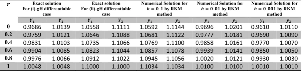
Table 2: Comparison of the exact solutions and numerical solutions by m Runge kutta Mersion method for different step lengths at = 0.1
Exact solution For (i)-gH differentiable
case
Exact solution For (ii)-gH differentiable
case
Numerical Solution for = . by RKM
method
Numerical Solution for = . by RKM
method
Numerical Solution for = . by RKM
method
0 0.9686 1.0139 1.0558 1.1111 1.0592 1.1144 0.9696 1.0201 0.9610 1.0110 0.2 0.9759 1.0121 1.0646 1.1088 1.0681 1.1122 0.9777 1.0181 0.9690 1.0090
0.4 0.9831 1.0103 1.0735 1.1066 1.0769 1.1100 0.9858 1.0161 0.9770 1.0070 0.6 0.9904 1.0085 1.0823 1.1044 1.0857 1.1078 0.9939 1.0141 0.9850 1.0050 0.8 0.9976 1.0066 1.0912 1.1022 1.0945 1.1056 1.0020 1.0121 0.9930 1.0030
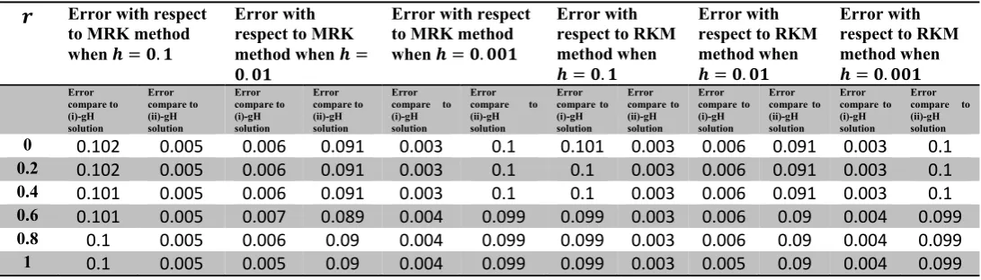
Table 3: The absolute error of approximating ( , ) on MRK and RKM method
Error with respect to MRK method when =
.
Error with respect to MRK method when
= .
Error with respect to MRK method when =
.
Error with respect to RKM method when = .
Error with respect to RKM method when = .
Error with respect to RKM method when
= . Error compare to (i)-gH solution Error compare to (ii)-gH solution Error compare to (i)-gH solution Error compare to (ii)-gH solution Error compare to (i)-gH solution Error compare to (ii)-gH solution Error compare to (i)-gH solution Error compare to (ii)-gH solution Error compare to (i)-gH solution Error compare to (ii)-gH solution Error compare to (i)-gH solution Error compare to (ii)-gH solution
0 0.0919 0.0047 0.001 0.0862 0.0076 0.0948 0.091 0.003 0.001 0.086 0.008 0.095
0.2 0.0935 0.0048 0.0018 0.0869 0.0069 0.0956 0.092 0.004 0.002 0.087 0.007 0.096
0.4 0.0951 0.0047 0.0027 0.0877 0.0061 0.0965 0.094 0.003 0.003 0.088 0.006 0.096
0.6 0.0966 0.0047 0.0035 0.0884 0.0054 0.0973 0.095 0.003 0.004 0.088 0.005 0.097
0.8 0.0983 0.0047 0.0044 0.0892 0.0046 0.0982 0.097 0.003 0.004 0.089 0.005 0.098
1 0.0999 0.0047 0.0052 0.09 0.0038 0.099 0.099 0.003 0.005 0.09 0.004 0.099
Table 4: The absolute error of approximating ( , ) on MRK and RKM method
Error with respect to MRK method when = .
Error with respect to MRK method when =
.
Error with respect to MRK method when = .
Error with respect to RKM method when
= .
Error with respect to RKM method when
= .
Error with respect to RKM method when = . Error compare to (i)-gH solution Error compare to (ii)-gH solution Error compare to (i)-gH solution Error compare to (ii)-gH solution Error compare to (i)-gH solution Error compare to (ii)-gH solution Error compare to (i)-gH solution Error compare to (ii)-gH solution Error compare to (i)-gH solution Error compare to (ii)-gH solution Error compare to (i)-gH solution Error compare to (ii)-gH solution 0 0.102 0.005 0.006 0.091 0.003 0.1 0.101 0.003 0.006 0.091 0.003 0.1
0.2 0.102 0.005 0.006 0.091 0.003 0.1 0.1 0.003 0.006 0.091 0.003 0.1 0.4 0.101 0.005 0.006 0.091 0.003 0.1 0.1 0.003 0.006 0.091 0.003 0.1
0.6 0.101 0.005 0.007 0.089 0.004 0.099 0.099 0.003 0.006 0.09 0.004 0.099 0.8 0.1 0.005 0.006 0.09 0.004 0.099 0.099 0.003 0.006 0.09 0.004 0.099
1 0.1 0.005 0.005 0.09 0.004 0.099 0.099 0.003 0.005 0.09 0.004 0.099
8. Application in Industry:
A tank initially contains 300 gals of brine which has dissolved in it lbs of salt. Coming into the tank at 3 gals/min is brine with concentration lbs salt/gals and the well stirred mixture leaves at the rate 3 gals/min. Let ( ) lbs be the salt in the tank at any time ≥ 0. Then ( )+
( ) = , ∈ [0,0.5] with (0) = . If the initial condition being modeled as fuzzy number
= (1,2,3) and = (1,2,4). Find solution at = 0.4.
Solution: For (i)-gH differentiable case the exact solution is
( , ) =(1 + )
100 1 + 99
( , ) =(2 − )
50 +
(148 − 49 ) 50
For (ii)-gH differentiable case the exact solution is
( , ) = −(149 − 149 ) + (−248 + 50 ) + (400 − 200 )
Table 5: Comparison of the exact solutions and numerical solutions by Modified-Runge-Kutta method for different step lengths at = 0.4
Exact solution For (i)-gH differentiable
case
Exact solution For (ii)-gH differentiable
case
Numerical Solution for = . by Modified
RK method
Numerical Solution for = . by Modified RK method
Numerical Solution for = . by Modified
RK method
0 0.9960 2.9882 2.5872 3.3928 1.1047 3.3141 1.0100 3.0301 1.0010 3.0030 0.2 1.1953 2.7890 2.6279 3.2723 1.3257 3.0932 1.2121 2.8281 1.2012 2.8028
0.4 1.3945 2.5897 2.6685 3.1519 1.5466 2.8723 1.4141 2.6261 1.4014 2.6026 0.6 1.5937 2.3905 2.7091 3.0314 1.7675 2.6513 1.6161 2.4241 1.6016 2.4024 0.8 1.7929 2.1913 2.7498 2.9109 1.9885 2.4302 1.8181 2.2221 1.8018 2.2022
1 1.9921 1.9921 2.7904 2.7904 2.2094 2.2094 2.0101 2.0201 2.0020 2.0020
Table 6: Comparison of the exact solutions and numerical solutions by Runge-Kutta-Mersion method for different step lengths at = 0.4
Exact solution For (i)-gH differentiable
case
Exact solution For (ii)-gH differentiable
case
Numerical Solution for = . by RK Mersian
method
Numerical Solution for = . by RK Mersian method
Numerical Solution for = . by RK Mersian method
0 0.9960 2.9882 2.5872 3.3928 1.1034 3.3101 1.0100 3.0301 1.0010 3.0030 0.2 1.1953 2.7890 2.6279 3.2723 1.3240 3.0894 1.2120 2.8281 1.2012 2.8028 0.4 1.3945 2.5897 2.6685 3.1519 1.5447 2.8687 1.4140 2.6261 1.4014 2.6026
0.6 1.5937 2.3905 2.7091 3.0314 1.7654 2.6481 1.6161 2.4241 1.6016 2.4024 0.8 1.7929 2.1913 2.7498 2.9109 1.9861 2.4274 1.8181 2.2221 1.8018 2.2022
1 1.9921 1.9921 2.7904 2.7904 2.2067 2.2067 2.0201 2.0201 2.0020 2.0020
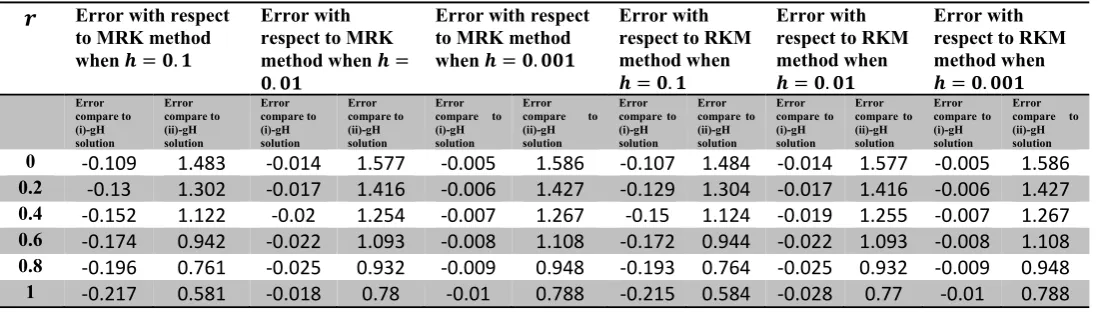
Table 7: The absolute error of approximating ( , ) on MRK and RKM method
Error with respect to MRK method when = .
Error with respect to MRK method when =
.
Error with respect to MRK method when = .
Error with respect to RKM method when
= .
Error with respect to RKM method when
= .
Error with respect to RKM method when = . Error compare to (i)-gH solution Error compare to (ii)-gH solution Error compare to (i)-gH solution Error compare to (ii)-gH solution Error compare to (i)-gH solution Error compare to (ii)-gH solution Error compare to (i)-gH solution Error compare to (ii)-gH solution Error compare to (i)-gH solution Error compare to (ii)-gH solution Error compare to (i)-gH solution Error compare to (ii)-gH solution 0 -0.109 1.483 -0.014 1.577 -0.005 1.586 -0.107 1.484 -0.014 1.577 -0.005 1.586
0.2 -0.13 1.302 -0.017 1.416 -0.006 1.427 -0.129 1.304 -0.017 1.416 -0.006 1.427 0.4 -0.152 1.122 -0.02 1.254 -0.007 1.267 -0.15 1.124 -0.019 1.255 -0.007 1.267
0.6 -0.174 0.942 -0.022 1.093 -0.008 1.108 -0.172 0.944 -0.022 1.093 -0.008 1.108 0.8 -0.196 0.761 -0.025 0.932 -0.009 0.948 -0.193 0.764 -0.025 0.932 -0.009 0.948
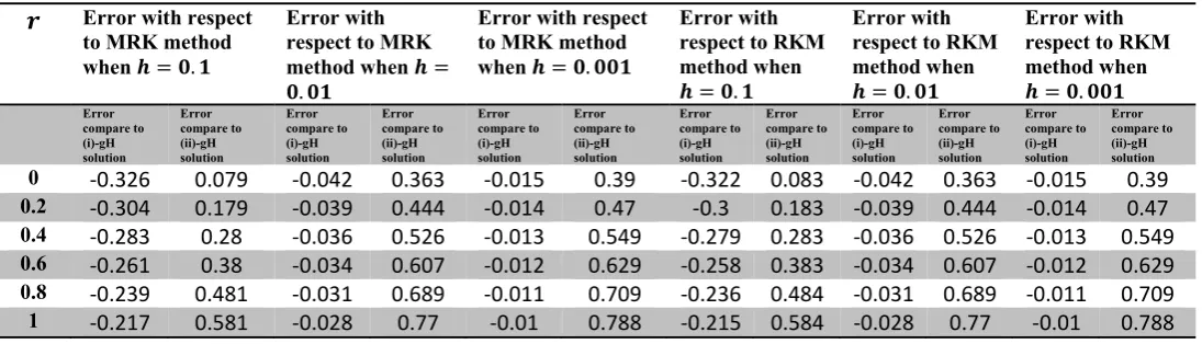
Table 8: The absolute error of approximating ( , ) on MRK and RKM method
Error with respect to MRK method when = .
Error with respect to MRK method when =
.
Error with respect to MRK method when = .
Error with respect to RKM method when
= .
Error with respect to RKM method when
= .
Error with respect to RKM method when = . Error compare to (i)-gH solution Error compare to (ii)-gH solution Error compare to (i)-gH solution Error compare to (ii)-gH solution Error compare to (i)-gH solution Error compare to (ii)-gH solution Error compare to (i)-gH solution Error compare to (ii)-gH solution Error compare to (i)-gH solution Error compare to (ii)-gH solution Error compare to (i)-gH solution Error compare to (ii)-gH solution 0 -0.326 0.079 -0.042 0.363 -0.015 0.39 -0.322 0.083 -0.042 0.363 -0.015 0.39 0.2 -0.304 0.179 -0.039 0.444 -0.014 0.47 -0.3 0.183 -0.039 0.444 -0.014 0.47
0.4 -0.283 0.28 -0.036 0.526 -0.013 0.549 -0.279 0.283 -0.036 0.526 -0.013 0.549 0.6 -0.261 0.38 -0.034 0.607 -0.012 0.629 -0.258 0.383 -0.034 0.607 -0.012 0.629 0.8 -0.239 0.481 -0.031 0.689 -0.011 0.709 -0.236 0.484 -0.031 0.689 -0.011 0.709
1 -0.217 0.581 -0.028 0.77 -0.01 0.788 -0.215 0.584 -0.028 0.77 -0.01 0.788
9. Remarks from above table on the solution
Our main aim is to compare the results between exact solution ((i)-gH and (ii)-gH) and two numerical methods namely Modified Runge Kutta method and Runge Kutta Mersion method on fuzzy differential equation. We show the comparison results between them with error estimation also. It is very difficult to consider the betterment of a method by solving a problem. In fuzzy case sometimes for different numerical example give different closure to exact solution. In crisp sense when we decrease the step length the numerical solution is tending to close to exact solution. But for fuzzy case it is happen not always.
10. Conclusion:
In this paper, Modified Runge Kutta Method and Runge Kutta Mersion method was taken into account to estimate the solution of first order linear ordinary differential equation with fuzzy initial condition, which is considered to be an important area of research with fuzzy differential equation. The approach generalized Hukuhara derivative concept, were applied to elucidate the exact fuzzy solutions of the given differential equation. Comprehensively, the whole deliberation reaches its conclusion with the following remarks:
• Demonstrating numerical methods for finding the solution of first order linear ordinary differential equation with fuzzy initial condition
• Compare the results with the exact solution which was found using generalized Hukuhara derivative approach.
• Numerical examples and application are taken to show for the importance of the mentioned numerical techniques.
• The accuracy for the result are discussed.
Conflict of Interests
The author declares that there is no conflict of interests.
Acknowledgement
The first author of the article wish to give the heartiest thanks to Miss. Gullu for giving inspiration to write this article.
References
[1] A. Kandel, W. J. Byatt, Fuzzy differential equations, in: Proceedings of International Conference Cybernetics and Society, Tokyo: (1978) 1213- 1216.
[2] E. Hüllermeier, An approach to modelling and simulation of uncertain systems, Int. J. Uncertain Fuzziness 5 (1997) 117–137.
[3] P. Diamond, Time-dependent differential inclusions, cocycle attractors and fuzzy differential equations, IEEE Trans. Fuzzy Syst. 7 (1999) 734–740.
[4] P. Diamond, Stability and periodicity in fuzzy differential equations, IEEE Trans. Fuzzy Syst. 8 (2000) 853– 890.
[5] P. Diamond, P. Watson, Regularity of solution sets for differential inclusions quasiconcave in a parameter, Appl. Math. Lett. 13 (2000) 31–35.
[6] B. Bede, S.G. Gal, Generalizations of the differentiability of fuzzy-number-valued functions with applications to fuzzy differential equations, Fuzzy Set Syst. 151 (2005) 581–599.
[7] B. Bede, I.J. Rudas, A.L. Bencsik, First order linear fuzzy differential equations under generalized differentiability, Inf. Sci. 177 (2007) 1648–1662.
[8] M. Chen, C. Wu, X. Xue, G. Liu, On fuzzy boundary value problems, Inf. Sci. 178 (2008) 1877–1892.
[9] C.Duraisamy, B.Usha, Numerical Solution of Fuzzy Differential Equations by Runge Kutta Method of Order three, International Journal of Advanced Scientific and Technical Research, Issue 1, Vol 1, Octobor 2011, ISSN 2249-9954.
[10] V.Nirmala,S.Chenthur Pandian, Numerical Solution of Fuzzy Differential Equations by Fourth order Runge Kutta Method with Higher Order Derivative Approximations, European Journal of Scientific Research, ISSN 1450-216X, No.2(2011),pp.198-206.
[11] T. Jayakumar, D. Maheskumar and K. Kanagarajan, Numerical Solution of Fuzzy Differential Equations by Runge Kutta Method of Order Five, Applied Mathematical Sciences, Vol. 6, 2012, no. 60, 2989 – 3002.
[12] B. Ghazanfari, A.Shakerami, Numerical solutions of fuzzy differential equations by extended Runge–Kutta-like formulae of order 4, Fuzzy Sets and Systems 189 (2011) 74–91.
[13] K. Kanagarajan, M. Sambath, Numerical solution of fuzzy differential equations by third order Runge-Kutta method, International Journal of Applied Mathematics and Computation Volume 2(4),pp 1-8,2010.
[14] T. Jayakumar, K. Kanagarajan, Numerical Solution for Hybrid Fuzzy System by Runge Kutta Fehlberg Method, Int. Journal of Math. Analysis, Vol. 6, 2012, no. 53, 2619 – 2632.
[16] Mojtaba Ghanbari, Solution of the first order linear fuzzy differential equations by some reliable methods, ISPACS, Volume 2012, Year 2012 Article ID jfsva-00126, 20 pages, doi:10.5899/2012/jfsva-00126.
[17] Nirmala.V, Chenthur Pandian.S, New Multi-Step Runge –Kutta Method For Solving Fuzzy Differential Equations, Mathematical Theory and Modeling, Vol.1, No.3, 2011.
[18] N.Saveetha, Dr.S.Chenthur Pandian, Numerical solution of Fuzzy Hybrid Differential Equation by Third order Runge Kutta Nystrom Method, Mathematical Theory and Modeling, Vol.2, No.4, 2012.
[19] N. M. Deshmukh, A new approach to solve Fuzzy differential equation by using third order Runge-Kutta method, ISSN No-2031-5063 Vol.1,Issue.III/Sept11pp.1-4.
[20] C. Duraisamy, B. Usha, Numerical Solution of Fuzzy Differential Equations by Runge-Kutta Method of Order Four, European Journal of Scientific Research, ISSN 1450-216X Vol.67 No.2 (2012), pp. 324-337.