The Impact of Government Expenditures on Unemployment: A Case Study of Jordan

THE

IMPACT

OF

GOVERNMENT

EXPENDITURES

ON

UNEMPLOYMENT: A CASE STUDY OF JORDAN

Shadi Saraireh PhD; Belarus State University of Economics, Associate Professor, Amman University College / Balqa Applied University Jordan.

ABSTRACT

Article History Received: 17 April 2020 Revised: 20 May 2020 Accepted: 25 June 2020 Published: 15 July 2020

Keywords: Jordan Government Spending Unemployment ARDL. JEL Classification: C51, E62, H50, O54.

In this paper, we estimate the effects of Government spending on unemployment in Jordan for the period 1990 to 2019. By using the ARDL co-integration test we found a negative and statistically significant long-run relationship between government spending and the unemployment rate in Jordan. An increase in government spending by a per cent of GDP is found to reduce unemployment by about 0.43 percentage points in the same year. We also noticed that, in the short-run, government spending has a positive and significant impact on unemployment.

Contribution/ Originality:

1. INTRODUCTION

The economic theory proposes a series of clarifications on the negative relationship between public spending and the unemployment rate. First, government spending excludes private spending, especially spending on investments that would increase efficiency and convince the change in production. In theory, public spending can be allocated to infrastructure and mentoring to increase growth, but in practice, most spending goes to government-determined reallocation or consumption, which does not improve productivity. Secondly, the level of public spending may impose other government interference in the operation of the private sector, specific guidelines that limit economic development and productivity.

Another ARDL investigation has shown that, as authorities spend, the increase in production will also boost higher. However, much research shows that tax cuts may have greater effects on production growth. According to Okun's law, production hurts unemployment. This means that when production increases, unemployment will decrease. There is also research indicating that as public spending increases, unemployment decreases. According to the results of these surveys, taxes will also have a major impact on unemployment.

Conducting an empirical study in Sweden can yield interesting results. Sweden has a long history of high taxes and remains one of the countries in the international world with the best tax burden. Furthermore, there is great

Asian Journal of Economic Modelling

ISSN(e):

DOI: 10.18488/journal.8.2020.83.189.203 Vol. 8, No. 3, 189-203.

consideration within the government among the population of Sweden. The model is an ARDL version with output, taxes, interest rate, spending and unemployment as established variables. Two trend variables are also protected in the VAR: a linear trend and a nonlinear shape. The information used in the analysis is Swedish quarterly records (“Statistics Sweden”) and Sweden's leading financial institution. The data is from 1994 to 2012.

According to business analysts, extensive financial strategy stirs work and diminishes joblessness. Existing investigations for the United States economy approve this customary perspective on Ravn and Simonelli (2007). Shockingly, the connection between open spending and joblessness stays vague because there is clashing experimental proof on the viability of money related motivations for joblessness. Monacelli, Perotti, and Trigari (2010) show experimental proof that financial motivations improve joblessness by applying an auxiliary investigation of VAR and constructs a reproducible co-incorporation model with relating erosion in the style of Mortensen and Pissarides (1994).

Brückner and Pappa (2012) show that financial extensions decline unemployment rate from a VAR auxiliary investigation and present another Keynesian form with relating rubbing that may clarify the test. Accordingly, our inquiries are sufficiently simple: Can financial boost or government spending improve joblessness? If this is true, what is the enormous increment in broad daylight spending that improves the unemployment rate?

Lack of openings for work intensifies the joblessness circumstance in which few people with employments, inside the workforce, with the vital capabilities, aptitudes and capacities are willing and searching for work. However, they can't look for some kind of employment (Adawo, Essien, & Ekpo, 2012). As per (Jhingan, 2008) insufficiency in openings for work prompts automatic joblessness of individuals who are eager to work with the triumphant pay, however, cannot get employment opportunity. The work arranges measure the extent of the accessible work power procured in the monetary framework (Nwosa & Emma-Ebere, 2017).

As indicated by observational proof from Holden and Sparrman (2013) government spending can expand the degree of business and lessen joblessness in each created and developing nation. Nonetheless, despite enormous government spending being spent on proficient divisions, for example, foundation, safeguard of citizenship, training, and wellbeing in Africa, there has been a consistent increment in the joblessness stage on the landmass.

Ram (1986) most current causality studies have reported that differences like the underlying statistics, the examination of the process, and duration studied can provide an additional explanation for the range of results. A few years later, Ahsan, Kwan, and Sahni (1992) added different variables to find a long and short-term relationship between public spending and unemployment. They found a positive relationship between public spending and unemployment in the short term, but in the long term, the connection between the variables was negative.

In the case of Nigeria, although investigations such as Momodu and Ogbole (2014) and Obayori (2016) attempted to examine the impact of monetary coverage on unemployment, they did not contain the two monetary policy provisions in their evaluation. They effectively included public spending and omitted revenue (important about financial coverage).

By definition, public or government spending is the expense incurred through public authorities such as the central, national, and neighbourhood governments to meet people's collective social needs (Grenade & Wright, 2012). Unemployment (or unemployment) occurs when humans are out of work and actively looking for paintings.

analysis also aims to find the long run as well as the short-run relationship between our dependent and independent variables through cointegration

2. LITERATURE REVIEW

The argument that higher work taxes are accountable for better unemployment amounts and it appears to be very appealing. In addition to many theoretical outcomes derived from static models, there is a broader view that higher taxes and unemployment have simultaneously increased during the seventies and eighties, and that Asian nations confirmed greater stages of each variable in evaluation to other economies, such with the China, wherein labour taxes and unemployment decreased. Lane and Perotti (1998) found that, inside the salary compensation issue of government, consumption reason significantly more grounded withdrawals in trades. According to Burgert and Gomes (2011) future potential issues of utilizing total information of administration spending to gauge its impacts on yield and different factors that take a gander at how changes in various specialists’ expenses proliferate in the economy.

Rocha and Divino (2002) studied the association among taxes on family expenditures and the unemployment rate in Brazil and Mexico. These researchers utilized the ARDL models and the results indicate that in both countries, the real interest rate is positively associated with unemployment, whereas taxes on family income are negatively associated with unemployment. Moreover, Yuan and Li (2000) dealt with the issue in a traditional Real Business Cycle model and found that using pressure on “why increasing government spending” may additionally push unemployment upwards. According to Ahsan et al. (1992) the public expenditure countrywide profits nexus, fail to account for overlooked variables which can supply upward push to deceptive causal ordering among variables and, in general, yields biased consequences.

Keynes in Sukirno (2002) states that the purpose or interference of the government is critical if the financial system is regulated via an unrestricted market, as the economy does no longer reach complete employment level nor it reaches such stability. One form of intervention is through monetary coverage. In this case, Keynes implies expansive monetary coverage through tax reductions and the addition of government expenditure.

Ramey (2011) found that the impacts of increments in government spending on utilization, unemployment, and genuine compensation bolster the consequences of the neoclassical model. The neoclassical model predicts that families diminish utilization and supply more work because of increments in government uses financed by single amount charges. For the time being, this lessens the balance of genuine pay and builds the peripheral item of capital. Loan fees rise, energizing an expansion in the venture; capital aggregates and the genuine compensation comes back to its steady-state level.

Moreover, McKay and Reis (2016) appear that redistributive arrangements, for example, unemployment rate, can have a significant effect in hosing total shocks when the fiscal approach doesn't completely react to variation in total activity. The fiscal approach is set at the national level and can't depend upon the nearby financial shock. They offer exact help for the unemployment rate as a stabilizer by seeing that utilization reacts less to antagonistic shocks in areas with the progressively liberal unemployment rate because the jobless have increasingly discretionary cash flow.

Zulhanafi, Aimon, and Syofyan (2013) endorse that national government spending appreciably impacts unemployment. If government expenditure increases, like capital expenditure to improve infrastructure, it's going to boom output, and the expanded output will boom the call for elements of manufacturing, one of which is employment; for this reason, this sort of situation might result in lowering the joblessness rate. Conversely, if government spending decreases, it's going to abate the manner of manufacturing of products and services output, so the demand for elements of manufacturing will also decrease inflicting the unemployment price to growth.

attention on sectoral expenses. The number one studies consequences showed that the share of government capital expenditure in a gross domestic product is definitely and drastically correlated with the financial increase, however, cutting-edge expenditure is insignificant. The result at the sectoral level discovered that government funding and general expenditures on schooling are the simplest outlays that stay substantially associated with growth for the duration of the analysis.

3. METHODOLOGY

The main purpose of this paper is to find a connection in both the short and long run between government expenditure and unemployment in Jordan. The first step is to check the data for stationarity hence we run the Augmented Dickey-Fuller (ADF) test. The first order ADF equation is given in Equation 1.

(1)

Where; is change in unemployment in time period t.

is income in time period 0.

is income government expenditure in time period t-1.

is income tax in time period 2.

is the error term.

Thus change in unemployment in period t is given by income in period 0 plus income government expenditure in period t-1 plus income tax in period 2 plus the error term

The ADF test for higher order is given in Equation 2.

(2)

Where; is unemployment rate in time period t.

is income in time period 0.

is income in time period 1*unemployment rate in time period t-2.

is income time period p-2*unemployment rate in time period t-p+2.

is income in time period p-1*unemployment rate in time period t-p+1.

is income in time period p*unemployment rate in time period t-p.

is the error term.

Thus unemployment rate in period t is given by income in time period 0 plus income in time period 1*Unemployment rate in time period t-1 plus income in time period 1*unemployment rate in time period t-2 plus income time period p-2*unemployment rate in time period t-p+2 plus income in time period p-1*unemployment rate in time period t-p+1 plus income in time period p*unemployment rate in time period t-p plus the error term.

In next step, we added and subtracted term to obtain.

(3)

Where; is unemployment rate in time period t.

is income in time period 0.

is income in time period 1*unemployment rate in time period t-1.

is income in time period 2*unemployment rate in time period t-2.

is (income in time period p-1 plus income in time period p)*unemployment

rate in time period-p+1.

is income in time period p* by change in unemployment in time period t-p+1

is the error term.

Thus unemployment rate in time period t is given by income in time period 2*unemployment rate in time period t-2 plus income in time period 2*unemployment rate in time period t-2 plus income in time period p-2*unemployment rate in time period t-p+2 plus (income in time period p-1 plus income in time period

p)*unemployment rate in time period-p+1 minus income in time period p* by change in unemployment in time period t-p+1 plus the error term

Next, add and subtract from Equation 3 we obtain:

(4)

Where; is unemployment rate in time period t.

is income in time period 0.

is income in time period 1*unemployment rate in time period t-1.

is income in time period 2*unemployment rate in time period t-2.

is (income in time period p-1 plus income in time period p)*unemployment

rate in time period-p+2.

is income in time period p* by change in unemployment in time period t-p+1.

is the error term.

(income in time period p-1 plus income in time period p)*unemployment rate in time period-p+2 minus income in time period p* by change in unemployment in time period t-p+1 plus the error term.

The final form of ADF model is given in Equation 5

(5)

Where and

Where; is change in unemployment rate in time period t.

is income in period 0.

is the standard deviation of unemployment rate in time period t-1.

is the summation proportion of change in unemployment rate in time period t-i+1

is the error term.

Thus change in unemployment rate in time period t is given by income in period 0 plus the standard deviation of unemployment rate in time period t-1 plus the summation proportion of change in unemployment rate in time period t-i+1 plus the error term.

In Equation 5 the coefficient of interest is ; if =0, and the equation is in stationary on first differences.

We can find this relationship by estimating the ARDL model. So, in next step, we will establish the ARDL methodology. The ARDL model for dependent variable (unemployment) and independent (government expenditure) variable is given in Equation 6.

(6)

Where; is unemployment rate in time period t.

is the summation proportion of unemployment rate in time period t-1.

is the summation of government expenditure in time period t-1.

is the schotastic term.

Thus unemployment rate in time period t is given by mean plus the summation proportion of unemployment rate in time period t-1 plus the summation of government expenditure in time period t-1 plus the schotastic term

(7)

Where is the unemployment rate in time period t.

is the mean.

is the proportion of unemployment rate in time period t-i.

is the proportion of unemployment in time period t.

is government expenditure * lambda in time period 0.

is government expenditure in time period t-1* .

is government expenditure in time period t-m * .

is the schotastic term.

Thus unemployment rate in time period t is given by mean plus the proportion of unemployment rate in time period t-I plus the proportion of unemployment in time period t plus government expenditure * lambda in time

period 0 plus government expenditure in time period t-1* plus government expenditure in time period t-m *

Where, UNEM is the unemployment rate and GEXP is the government expenditure. The term “t” is the time

period and is the error term. The key aim of this study is to get the long-term coefficient values of both UNEM

and GEXP. So, the basic idea is to calculate the steady state level of and , the steady state form is

given in Equation 8:

(8)

Let assume is constant

(9)

In next step, we substituted the Equation 9 into Equation 6 to find a long run coefficient

(10)

or

(11)

The basic goal is to find both short-run and long-run coefficients and we can get long-run coefficients by assessing the Equation 12.

(12)

Where; is the change of unemployment rate in time period t.

is the mean.

is the summation of change in unemployment rate in time period t-i.

is the standard deviation in time period 1* unemployment rate in time period t-1.

is the standard deviation in time period 2* the government expenditure.

is the error term in time period t.

Thus change of unemployment rate in time period t is given by the mean plus the summation of change in unemployment rate in time period t-I plus the summation of change in government expenditure in time period t-1 plus the standard deviation in time period 1* unemployment rate in time period t-1 plus the standard deviation in time period 2* the government expenditure plus the error term.

The and variables state the long-term parameters in the autoregressive distribution lag

(ARDL) model (Enders, 2015).

4. DATA AND VARIABLES

We employ time-series data between the period of 1990 and 2019 collated from World Bank (WDI). The region of analysis is Jordan. A total of five dependent and independent variables are used in this study. The dependent variable is the unemployment rate and the independent variables are Private investment (PINV), Official development assistance (ODA), Gross fixed capital formation (GFCF), and employment opportunities (EMOP).

Table-1. Statistics summary results.

Statistics UNEM PINV GEXP ODA GFCF EMOP

Mean 15.088 84.542 20.254 27.680 23.883 6.443

Median 14.650 88.159 21.137 24.024 23.765 6.416

Maximum 21.951 89.817 25.194 86.604 33.088 6.689

Minimum 11.900 71.150 15.271 10.946 17.774 6.128

Std. Dev. 2.632 6.057 3.410 17.961 4.414 0.174

Skewness 1.246 -0.928 -0.251 1.9281 0.339 -0.164

Kurtosis 3.803 2.337 1.592 6.3942 1.918 1.686

Jarque-Bera 8.570 4.856 2.7905 32.989 2.040 2.291

Probability 0.013 0.088 0.2477 0.000 0.360 0.317

Observations 30 30 30 30 30 30

The summary statistics are given in Table 1. A total of thirty observations are included in our data set. The mean value of the unemployment rate between the period of 1990 and 2019 is 15.09%. The maximum unemployment rate value in Jordan is 21.95 between the period of1990 and 2019 and the minimum value is 11.90. Both skewness and kurtosis values of unemployment rate data are positive.

4.1. Augmented Dicky Fuller Stationarity Test

To estimate a relationship between the unemployment rate and government expenditure the first thing we need do check is either our data set has a unit root or not.

So, we ran an ADF test to check the stationarity of the data and results are given in Table 2.

0.01 on the level. The remaining three variables are stationary on the level. We concluded that, some variables are stationary on level and some variables has a unit root on first difference. So, we can use ARDL test because series has a combination of both level and first difference data stationarity.

Table-2. Unit root ADF test.

H0: Series is stationary

Level I (0) First Difference I (1)

Intercept and Trend P-value Intercept and Trend P-value

UNEM -1.372 0.847 -5.204 0.001

GEXP -2.315 0.413 -5.544 0.000

PINV -5.986 0.000 -5.216 0.002

ODA -3.440 0.065 -6.825 0.000

GFCF -2.159 0.492 -4.746 0.003

EMOP -7.771 0.000 -13.936 0.010

Note: 1%, 5% and 10% represent the ***, ** and * significance level.

In the next step, we will check either co-integration exists between the dependent and independent variables. We ran abound F-statistics test for this and results can be seen from Table 3.

Table-3. F-bounds test.

F-statistic 11.7269

Significant level I (0) I (1)

a-=10% 2.08 3

a=5% 2.39 3.38

a=2.5% 2.7 3.73

a=1% 3.06 4.15

If the calculated F-statistic value falls underneath the lower bound we would conclude that the variables are I (0), so no cointegration exits in this case. If the F-statistic value exceeds the upper limit I (1), we finish that we've cointegration. Finally, if the statistic falls among both limits, the test is inconclusive. In our case, the Bound F-statistics value is (11.7269) which is greater than both the lower and upper limit. So, we concluded that the long-run association occurs between dependent and independent variables.

5. EMPIRICAL FINDINGS

In this chapter, we estimate both long and short-run coefficient and the results of long-run parameters are given in Table 4. According to the results, there is a negative relationship between the unemployment rate and government expenditure.

Table-4. ARDL Long run Coefficients (1, 0, 1, 2, 0, 0).

Variable Coefficient

GEXP -0.407** _-0.192

PINV -0.251** _-0.098

ODA 0.134*** _-0.028

GFCF -0.213* _(-2.034)

EMOP 12.500** _-2.242

C -51.149 _(-1.489)

The relationship between both variables is statistically significant at the level of 5%. It means that, when the government spends more, then more jobs will be created and unemployment will be decreased. The GEXP coefficient value is -0.407, which implies that if government expenditure increases by one percent unemployment rate will decrease by 0.4072 percent. The relationship between private investment and unemployment rate is negative and statistically significant.

The findings suggest that ODA harms the unemployment rate which we attributed to corruption and funds not been allocated properly. GFCF has a negative but statically significant connection with the unemployment rate. If GFCF increases by one unit the value of unemployment will be decreased by 0.21 units.

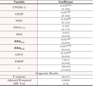
On the other hand, there is a positive relationship existing between unemployment and government expenditure in short-run Table 5. It means that in short term government expenditure harms unemployment and this can be attributed to the crowding out effects of government. The private investment has a negative relationship with unemployment in both short and long run.

Table-5. ARDL short run coefficients (1, 0, 1, 2, 0, 0).

Variable Coefficient

UNEM(-1) 0.416*** _(0.102)

GEXP 0.237** _(0.102)

PINV -0.340** _(0.135)

PINV(-1) _(0.115) 0.193

ODA _(0.016) -0.015

0.025** (0.010) 0.067***

(0.012)

GFCF -0.124** _(0.052)

EMOP _(2.956) 7.2911

C _(18.624) -29.833

Diagnostic Results

F-statistic 30.074

Adjusted R-squared

DW Test 0.9064 2.72

The GFCF has a positive connection with UNEM in short run. The R-squared value explains how well the regression model fits the observed data. In our case, the R-squared value is 0.9376, which reveals that 93.76 % of the data fit the regression model and remaining counts as an error term.

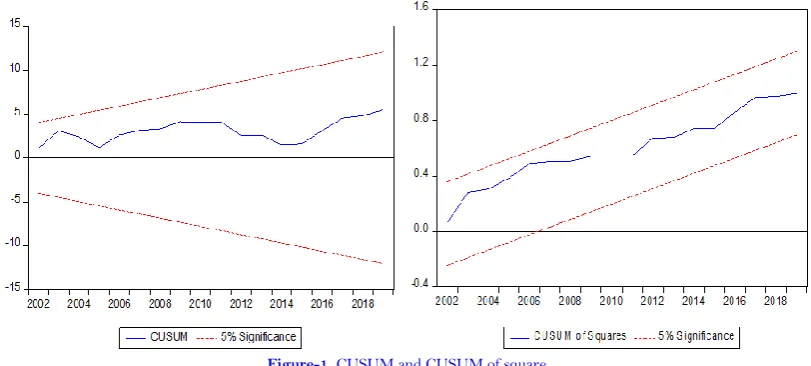
Figure-1. CUSUM and CUSUM of square.

Finally, we verified the cumulative sum tests (CUSUM) and CUSUM of squares (CUSUMSQ), used to verify the stability of the structure in the model and which can be seen in Figure 1. The results explain that the equilibrium of government spending and unemployment coefficient is stable over time because both the red line is within the range, where stability is a requirement to use this model for sample prediction. The results support the result of the variance equation of the ARDL estimates and decrease persistence in the Jordanian economy.

6. CONCLUSION

In theoretical literature, we concluded that lack of job opportunities intensifies the unemployment situation in which some people with jobs, within the workforce, with the necessary qualifications, skills and abilities are willing and looking for work, but cannot find work. Jordan government, like other Asian developing countries, wants to reduce the unemployment rate because the country is a labor-intensive country.

Informed by the widely revised literature, an increase in unemployment will constantly lessen cumulative production and, therefore, slow development. The short-time period results showed that public spending and unemployment are related; this means that Jordan is more consumer-susceptible, so any boom in recurrent spending will increase the unemployment rate and generally tend to lower economic happiness.

In this paper, we found that long-run unemployment decreases if the government spends more on infrastructure, health, and education. We also found a negative relationship between government spending and unemployment. Secondly, we found that Jordan private sector could reduce the unemployment rate if the government provides ease of doing business opportunities on an equal basis. The private sector also reduces the output gap and will also increase the aggregate demand in an economy.

Funding: This study received no specific financial support.

Competing Interests: The author declares that there are no conflicts of interests regarding the publication of this paper.

REFERENCES

Adawo, M., Essien, E., & Ekpo, N. (2012). Is Nigeria. Current Research Journal of Social Sciences, 4(6), 389-395.

Ahsan, S. M., Kwan, A. C., & Sahni, B. S. (1992). Public expenditure and national income causality: Further evidence on the role of omitted variables. Southern Economic Journal, 58(3), 623-634.Available at: https://doi.org/10.2307/1059830. Akrani, G. (2011). What is public expenditure? Meaning and classification. Retrieved from

https://kalyan-city.blogspot.com/2011/02/what-is-public-expenditure-meaning-and.html.

Burgert, M., & Gomes, P. (2011). The effects of government spending: A disaggregated approach. Paper presented at the Contributions to the Annual Meeting of the Association for Social Policy 2011: The Order of the World Economy: Lessons from the Crisis - Session: Fiscal Stimulus, No. G2-V3, ZBW - German Central Library for Economics, Leibniz Information Center for Economics.

Enders, W. (2015). Applied econometric time series (4th ed., pp. 118-174). Hoboken, NJ: Wiley.

Grenade, K., & Wright, A. (2012). The relationship between public spending and economic growth in selected caribbean

countries: A re-examination. Retrived from

https://www.cbvs.sr/ccmf/index_files/ccmf_papers/Public%20spending%20and%20economic%20growth_Kari%20G renade.pdf.

Holden, S., & Sparrman, V. (2013). Do government purchases affect unemployment? Retrived from https://core.ac.uk/download/pdf/193221687.pdf.

Jhingan, M. L. (2008). Macroeconomic theory. India: Vrinda Publications (P) Ltd.

Josaphat, P. K., & Oliver, M. (2000). Government spending and economic growth in Tanzania, 1965-1996. Credit Research Paper, Centre for Research in Economic Development and International Trade University of Nottingham, 00-6. Lane, P. R., & Perotti, R. (1998). The trade balance and fiscal policy in the OECD. European Economic Review, 42(3-5), 887-895. McKay, A., & Reis, R. (2016). The role of automatic stabilizers in the US business cycle. Econometrica, 84(1), 141-194.

Momodu, A. A., & Ogbole, O. F. (2014). Public sector spending and macroeconomic variables in Nigeria. European Journal of

Business and Management, 6(18), 232-243.

Monacelli, T., Perotti, R., & Trigari, A. (2010). Unemployment fiscal multipliers. Journal of Monetary Economics, 57(5),

531-553.Available at: https://doi.org/10.1016/j.jmoneco.2010.05.009.

Mortensen, D. T., & Pissarides, C. A. (1994). Job creation and job destruction in the theory of unemployment. The Review of

Economic Studies, 61(3), 397-415.Available at: https://doi.org/10.2307/2297896.

Nwosa, P. I., & Emma-Ebere, O. O. (2017). The impact of financial development on foreign direct investment in Nigeria. Journal of Management and Social Sciences, 6(1), 181-197.

Obayori, J. B. (2016). Fiscal policy and unemployment in Nigeria. The International Journal of Social Sciences and Humanities

Invention, 3(2), 1887-1891.

Ram, R. (1986). Government size and economic growth: A new framework and some evidence from cross-section and time-series data. The American Economic Review, 76(1), 191-203.

Ramey, V. A. (2011). Identifying government spending shocks: It's all in the timing. The Quarterly Journal of Economics, 126(1), 1-50.Available at: https://doi.org/10.1093/qje/qjq008.

Ravn, M. O., & Simonelli, S. (2007). Labor market dynamics and the business cycle: Structural evidence for the United States. Scandinavian Journal of Economics, 109(4), 743-777.Available at: https://doi.org/10.1111/j.1467-9442.2007.00520.x. Rocha, C. H., & Divino, J. A. C. (2002). The determinants of unemployment in Brazil and Mexico. Economia, 3(2), 303-315. Sukirno, S. (2002). Introduction to macroeconomic theory (2nd ed.). Jakarta: PT. Raja Grafindo Persada.

Yuan, M., & Li, W. (2000). Dynamic employment and hours effects of government spending shocks. Journal of Economic

Dynamics and Control, 24(8), 1233-1263.Available at: https://doi.org/10.1016/s0165-1889(99)00007-x.

APPENDIX

Table-6. Harvey test for heteroskedasticity.

Model F-statistic 1.9736 Prob. Value 0.1050

Table-7. Ramsey REST test.

Model F-statistic 0.0057 Prob. Value 0.9407

Table-8. Multi-collinearity (variance inflation factors)test

Variable Variance VIF

UNEM(-1) 0.010490 3.937676

GEXP 0.010493 8.009833

PINV 0.018300 3.630865

PINV(-1) 0.013272 3.294696

ODA 0.000273 2.327627

ODA(-1) 0.000113 2.051557

ODA(-2) 0.000151 3.613707

GFCF 0.002733 3.952910

EMOP 8.741987 1.411853

C 346.8784 NA