N
EURONAL
N
ETWORKS
Thesis by
Shreesh Pranesh Mysore
In Partial Fulfillment of the Requirements
for the Degree of
Doctor of Philosophy
California Institute of Technology
Pasadena, California
2007
Acknowledgements
My journey to a Ph.D. has been via the scenic route – challenging and a tad long, but immensely enjoyable with a wide variety of research experiences and several wonderful mentors. Consequently, I have many people to thank.
I sincerely thank Prof. Erin Schuman, my adviser on the experimental part of this thesis, for her surprisingly, to me, great belief in my ability. When I first showed up in her office three years ago, Erin accepted my complete lack of experience in experimental biology at that time without so much as a hint of hesitation and permitted me to join her lab. The underlying philosophy of her lab to pursue any question of interest in neuroscience without constraints embodies wonderfully the fundamental spirit of the scientific quest and has facilitated an exciting, fun, and stimulating research experience. Without her support and guidance, I would never have started on the path of experimental neuroscience, a field that continues to fascinate me to no end, and one that I wish to make my academic home. She has repeatedly encouraged me when I least expected it, and has been a great research mentor. Her deep insight and incisive intellect are qualities I aspire to.
the computational modeling projects in my thesis were originally suggested by him. I have been repeatedly inspired by his ideas, his openness, his ability to motivate, and his desire to nurture the careers of young researchers. If not for Steve, I would not be here now, writing my Ph.D. thesis.
I am very thankful to Prof. Christof Koch in whose lab I worked for nearly a year and a half. At a critical juncture, he suggested a course-correction for me that, in hindsight, was a much needed one. I was too close to a problem to see it, but he gently suggested a solution and nudged me in the right direction. For this, and for his endless enthusiasm for science, I am very grateful.
I am extremely thankful for, and constantly astonished by, the breadth of the vision of the Control and Dynamical Systems (CDS) option at Caltech. Beginning with my application to this program, my research interests have never been within what some may consider as being the boundaries of a rigorous applied mathematics type program. Yet, since the first time I visited Caltech as a prospective, and all through the ups and downs of my graduate experience at Caltech, CDS, and particularly Prof. Richard Murray, have always encouraged my interests wholeheartedly. I have encountered no boundaries at all as I have tried to cross imaginary ones across research fields, and there are few other universities and departments where I could have expected broad-mindedness to such an extent, and such an inviting and invigorating research atmosphere. In hindsight, my decision to come here (over MIT) is one I would make again in a heartbeat. To Prof. Murray, CDS, and Caltech, I owe a great debt of gratitude.
while in his lab, and without that, I would not be able to appreciate so much of what I now can. When I was still an undergraduate, it was his research that inspired me to embark on the quest to understand, model, and design learning and intelligence. I was a clueless senior when he called up my home in Chennai to offer me a spot in his research group, and in the three years I spent in his lab, I learned so much about research, science, mentoring, and the passionate pursuit of science and engineering. For Dr. Kumara’s inspiring research, for excellent academic guidance, for the total academic freedom he allowed, and for his wonderful and warm heart, I cannot thank him enough. A truly wise person is Dr. Kumara, and I will be happy if I am even half of who he is, academically, and otherwise.
Also at Penn State, I was greatly influenced by Prof. Asok Ray. He served more as a mentor than as the instructor of several wonderful Math classes. A better teacher I have yet to encounter. His passion for understanding phenomena at a fundamental level and for solving problems influences all who work with him. A deep thinker, and a rigorous scientist, he continues to be one of my role models.
Before Penn State, there was IIT Madras. The seeds for my academic interest in all things to do with learning and intelligence were sowed during a year-long series of lectures on artificial neural networks by Prof. B. Yegnanarayana. I was still an undergraduate in Mechanical Engineering then, and these graduate classes in Computer Science riveted my attention like no other classes had in my entire four years. I thank him for teaching the subject so well and with such obvious zeal for the field.
favorites and I owe many thanks to their authors – Hermann Hesse for Siddhartha and Narcissus and Goldmund, Paulo Coelho for The Alchemist, and Plato for The Republic.
For as long as I can remember, I have always wanted to be an academic, and for this, I have my dad, Prof. M. R. Pranesh, to thank. His incredible intellect, unwavering integrity, unflinching discipline, and remarkable simplicity have molded me all my life. Thanks, dad, for instilling in me a desire for excellence, and for being there in ways I still don’t fully appreciate. My mom, Mrs. Rama Pranesh, gets almost all the credit for who I am today. For her wonderful patience, wisdom, understanding, and for choosing to raise us full-time, I cannot thank her enough; if not for her, I would be nothing. Of all her wonderful gifts to me, the greatest is music – a love for it, and an appreciation of its ability to uplift one’s soul. If I were not an aspiring academic, I would most certainly be an aspiring musician, all thanks to her. My sister, Dr. M. P. Veenashree has been a lighthouse for me all my life – always there, always guiding, always urging me to reach higher, and be wiser. From my earliest memory, she has been my best friend and someone who has understood me better than I have done myself. Thanks, sis!
Abstract
A. Responses in a normal network...91
B. Plasticity upon exposure to prism ...93
C. Predictions...98
4.6 CONCLUSIONS...98
4.7 FUTURE DIRECTIONS...99
CHAPTER 5. GENERAL DISCUSSION...100
5.1 N-CADHERIN, SPINE DYNAMICS, AND STRUCTURAL PLASTICITY...100
5.2 ARCHITECTURAL PLASTICITY AND REPRESENTATION CONSTRUCTION: BARN OWLS AND BEYOND...101
The average human brain has approximately 1011 neurons (Kandel et al., 2000) that are networked following a well-defined connectivity diagram. Each connection between a pair of neurons is called a synapse, and there are on the order of 1014 synapses (Shepherd, 1998; Tang et al., 2001). Information is thought to be encoded in the brain in a distributed fashion across these synapses. The encoded information, while stable, is also susceptible to change, or plasticity, to adapt to new environments and to learn new information. Two broad categories of neural plasticity can be distinguished based on how the changes are implemented in the brain. If the changes involve modifications to the network topology (or connectivity pattern), they are said to constitute architectural plasticity. If there is no change to the connectivity pattern, but the efficacies of existing functional synapses are modified, then there is said to be synaptic plasticity. Most forms of architectural plasticity involve structural changes – to spines, axons, dendrites, and neurons (the one exception is the unsilencing of preexisting, non-functional synapses (see Atasoy and Kavalali, 2006; Gasparini et al., 2000; Groc et al., 2006 for reviews). Though structural changes can accompany synaptic plasticity (e.g., changes to size and morphology of spines), there are numerous other, non-structural mechanisms as well that implement synaptic efficacy change.
dendritic spine motility (which includes the addition and elimination of functional spines), through axogenesis, the growth of new axonal branches to aid in the process of spinogenesis, and all the way to a change in the number of neurons, architectural plasticity in neuronal networks manifests itself as a spectrum of change ranging from the subtle to the drastic. In addition to being observed during development, the above mechanisms have been observed in adult brains as well. The most common mechanism of architectural plasticity in the brain appears to be dendritic spine motility. In this thesis, we will study structural plasticity in the brain and, particularly, its role in mediating architectural changes. In the rest of this chapter, will briefly describe the terminology used, review what is known about the different forms of architectural plasticity with an emphasis on spines, and summarize the remainder of the thesis.
1.1 Background
A. Synaptic communication
Neurons communicate with one another through electrical and chemical signals at specialized punctate structures called synapses. Typically, a synapse is formed between the output process (called axon) of one neuron and the input process (called dendrite) of another.1 Consequently, the axonal terminal is referred to as being pre-synaptic and the dendritic terminal, post-synaptic, and such a synapse is called axodendritic.2 Synapses can also be classified as being electrical or chemical based on the manner in which information is transmitted across them (Kandel et al., 2000).
1 Each neuron has a single axon, but numerous dendrites. Axons are much thinner than dendrites, which are also studded with spines in many cases.
Electrical synapses or gap junctions allow for the direct exchange of ions between neurons, and the resulting ionic current directly couples the electrical activity of one cell to that of the other. At chemical synapses, information is transmitted by the release of chemical factors called neurotransmitters. Neurotransmitters diffuse across the extracellular space connecting the pre- and post-synaptic terminals (called the synaptic cleft), are recognized by specialized proteins called receptors, and result in the opening of ion channels that allow the inward or outward flow of ions from the cell. The resulting ionic currents and post-synaptic voltage changes constitute the received signal. Neurotransmitter molecules are packaged in the pre-synaptic terminal in containers called synaptic vesicles and their release occurs by a process called exocytosis in which the vesicle fuses with the pre-synaptic membrane, opens up (partially or fully), and delivers its contents into the synaptic cleft. Release of neurotransmitter at the pre-synaptic site can be evoked by relatively large electrical spikes called action potentials or can be spontaneous. Finally, based on whether they increase or decrease the activity of the target neuron, synapses can be classified as being either excitatory or inhibitory.3 Excitatory synapses outnumber inhibitory ones (approximately 5:1 in the cat visual cortex (Shepherd and Koch, 1998)) and are usually formed on dendrites, whereas inhibitory synapses are formed on the cell body.4
3 More locally, synapses can be defined as excitatory or inhibitory based on the sign of the ionic current (with respect to the resting state of the target cell) at the post-synaptic site.
B. Spines
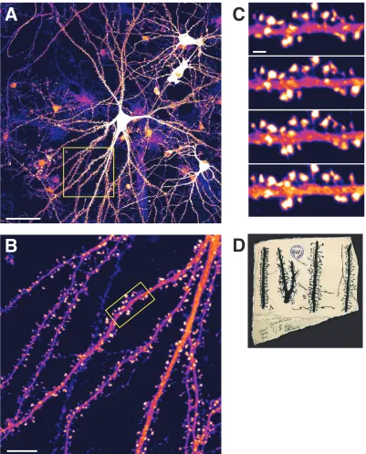
Spines are small morphological specializations that protrude from neuronal dendrites5 and were first described by Ramón y Cajal in 1888 in the cerebella of birds (see Bonhoeffer and Yuste, 2002). Most excitatory synapses (>90%) are formed on spines6 (Peters et al., 1991), and while some inhibitory synapses can be found on spines as well, typically, an inhibitory axospinal synapse is accompanied by an excitatory synapse on the same spine (Micheva and Beaulieu, 1995; Zito and Svoboda, 2002). Based on the synaptic input they receive, spines trigger different signaling pathways that can result in short-term or long-term synaptic changes. There are estimated to be more than 1013 spines in the human brain (Nimchinsky et al., 2002). A hippocampal pyramidal neuron (from rat) imaged live7 at 40x using a confocal microscope is shown in Fig. 1-1A, and a close-up of the boxed area is in Fig. 1-1B. Almost all the processes seen are dendrites, and the mushroom-like projections from them are spines. A time-lapse series of images of the boxed area in Fig. 1-1B illustrate that spines are morphologically dynamic (Fig. 1-1C). Cajal's drawings of spines are shown in Fig. 1-1D. Spines usually consist of a head (volume ~0.001–1 m3) that is connected to the dendrite by a neck, and spine lengths vary between 0.5 and 2 m.
5 Spines can be found on cell bodies and on initial axonal segments as well. 6 In other words, most axodendritic synapses are in fact axospinal.
A
B
C
D
Figure 1-1. Representative pyramidal neuron from rat hippocampus showing numerous dendritic spines.
(A) A hippocampal pyramidal neuron overexpressing GFP-actin8 virus and imaged at 40x. Scalebar = 50 µm. (B) Zoomed-in view of the boxed area in (A) with a closer view of dendritic spines. Scalebar = 10 µm. (C) Time-lapse images of the dendritic portion
boxed in (B) showing morphological dynamics in dendritic spines. Images are taken once every 5 minutes. Scalebar = 2 µm. (D) Drawings of different types of spines by Cajal circa 1891 (reproduced from Yuste, 2000). In (A)–(C), the intensity of GFP-actin is represented using the “fire” pseudo-coloring scheme from IMAGEJ. In this scheme, an intensity of 0 is represented by the color black, 255 by white, and intermediate intensities by shades of purple and pink.
C. Classification of spines
Detailed anatomical studies using electron microscopy have led to the
classification of dendritic protrusions into five types (Harris et al., 1992; Peters and
Kaiserman-Abramof, 1970): Type I are called stubby spines; Type II, mushroom-shaped
spines; Type III, thin spines; Type IV, filopodia; and Type V are called cup-shaped
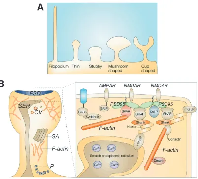
spines. Fig. 1-2A shows a schematic representation of these five types. If L, dh, and dn,
denote the spine length, head diameter and neck diameter, respectively, the rules used to
classify spines are: Type I if L~ dn ~ dh, Type II if dh >> dn, Type III if L>>dn, and Type
IV if L>5µm. Spine lengths are under 2 m, while filopodia can be up to 10 m.
Filopodia are also very thin and are sometimes called headless spines. As we will see
below, due to spine morphological dynamics in live neurons (Dailey and Smith, 1996),
and the transitions observed in spine shapes (Dunaevsky et al., 1999; Maletic-Savatic et
al., 1999; Parnass et al., 2000), the morphological label of a spine is dynamic as well.
D. Composition of spines
The subcellular composition of different kinds of spines (and filopodia) is diverse
(Hering and Sheng, 2001). Of the various components in spines, three are of most interest
to our discussion. They are actin (filamentous cytoskeletal element), an electron-dense
macromolecular complex of proteins called the post-synaptic density (PSD), and
these and other components subcellular components. The presence of actin in spines was determined early on (Fifkova and Delay, 1982) and its critical role in spine dynamics established (Fischer et al., 1998; Matus, 2000). Actin polymerization serves as the end effector that physically produces spine morphological changes. The PSD is perhaps the most important functional organelle in spines as it contains PSD95 (a major component that has been the subject of intense study (see Kennedy, 2000), and various neurotransmitter receptors, and communicates with several intracellular signaling mechanisms.9 Typically, it occupies about 10% of the area of the spine (Hering and Sheng, 2001). Polyribosomes are generally found at the base of spines. Various reviews discuss the structure and components of spines in detail (Hering and Sheng, 2001; Sorra and Harris, 2000).
A
B
Figure 1-2. Morphological classification and subcellular composition of dendritic spines.
(A) Morphological spine types: stubby spines (Type I), mushroom spines (Type II), thin spines (Type III), filopodia (Type IV) and cup-shaped spines (Type V) (adapted from Hering and Sheng, 2001). (B) Morphological classification of spines. PSD – post-synaptic density, P – polyribosomes, SA – spine apparatus, SER – smooth endoplasmic reticulum (adapted from Hering and Sheng, 2001).
1.2 Structural mechanisms of architectural plasticity
A. Spine motility
rats (Dailey and Smith, 1996; Fischer et al., 1998). Since its discovery, one of the main functions attributed to motility is that of exploring the extracellular space in search of pre-synaptic partners (but also see Dunaevsky et al., 2001). Other attributed functions are the modulation of biochemical signaling and protein scaffolding (Halpain, 2000). Motility has also been found in response to electrical stimulation of neurons (Maletic-Savatic et al., 1999), thus suggesting that experience may regulate motility. Direct evidence for this is available from several studies in which sensory deprivation of different kinds (tactile and visual) resulted in changes in spine dynamics, including effects on synapse turnover (Grutzendler et al., 2002; Holtmaat et al., 2006; Holtmaat et al., 2005; Lendvai et al., 2000; Majewska and Sur, 2003; Mizrahi and Katz, 2003; Trachtenberg et al., 2002; Zuo et al., 2005). These data, along with theoretical interpretations (Chklovskii et al., 2004; Poirazi and Mel, 2001; Stepanyants and Chklovskii, 2005) are strong evidence for spine dynamics as a potential mechanism driving architectural plasticity.
B. Changes in spine density and synapse number
spine density increase was blocked as well. Spatial training of rats, which is known to produce an increase in their subsequent ability to learn in spatial tasks, also produces an increase in the density of spines in the hippocampus (Moser et al., 1997). Other tasks like odor discrimination training (Knafo et al., 2001), visual stimulation, and even space flight (Yuste and Bonhoeffer, 2001), have been found to produce spine density increases in the appropriate brain regions in rats. A case can thus be made that experience-dependent plasticity in dendritic spines may facilitate architectural reorganization of neural circuits in response to functional demands.
changes, in adult neuronal tissue following physiologically relevant stimuli and learning paradigms.
C. Neurogenesis
Neurogenesis, like synaptogenesis and spine density changes, has been correlated with learning experiences. For instance, trace eye-blink conditioning and spatial learning in animals lead to an increase in the number of hippocampal neurons through an extension of neuronal lifetimes (Gould et al., 1999). There appears to be a critical period following cell production such that learning occurring in this period increases neuronal lifespan. In parallel, stressful experiences that result in a downregulation of cell proliferation in the dentate gyrus (Gould and Gross, 2002) are implicated in lower performance in hippocampally dependent learning tasks, suggesting a causal link between the two. Several conditions that increase neurogenesis (enriched environments, increased estrogen levels, wheel running, etc.) in mice and rats also enhance performance (Gould and Gross, 2002). Similarly, increases in social complexity have been found to enhance the survival of new neurons in birds (Lipkind et al., 2002). Finally, it has been found that the physiological properties of adult-generated granule cells in the dentate gyrus of the hippocampus resemble those of granule cells in young rats (Overstreet-Wadiche et al., 2006). This suggests that adult-generated neurons may share some properties with embryonic and early post-natal neurons in their ability to extend axons, form new connections more readily, and make more synapses. These characteristics may make adult neurogenesis an attractive “feature,” rather than a developmental “bug” in neuronal circuits.
1.3 Architectural plasticity and representation
construction
Formal learning theory. Formal learning theory (FLT) deals with the ability of a learner to arrive at a target concept based on examples of the concept. Three typical features of FLT models are that the learning algorithm searches through a predefined space of candidate hypotheses (concepts), it is expected to learn the concept exactly, and no restrictions are placed on the actual time taken by the learner to arrive at the target concept. FLT is therefore interested in “exact" and “in-principle” learnability, and the expectation is that generalization – a measure of performance on novel examples – is achieved. The classical formulation of FLT is discussed in the context of language learning by Gold (Gold, 1967). The key insight from formal work on language learning is that the learner must utilize a highly restricted set of all possible concepts in order to have even the possibility of generalizing. In other words, far from employing a general learner, from this perspective a language learning system must be meticulously tailored to the problem at hand, either by the designer in the case of artificial systems, or presumably by evolution in the case of biological learners.
the examples correctly with probability 1-, for arbitrarily small and . Nevertheless, the hypothesis space is still fixed a priori. A fixed hypothesis space yields such problematic theoretical issues as Fodor's paradox (Fodor, 1980), which states that nothing can be learned that is not already known; hence nothing is really learned. The idea here is that no hypothesis that is more complex than the ones in the given hypothesis space can be evaluated and hence learned. Therefore, all concepts need to be available in the hypothesis space before the search begins.
Constructive learning and architectural plasticity. Constructive learning (Piaget, 1970; Piaget, 1980; Quartz, 1993; Quartz and Sejnowski, 1997) addresses this issue of a fixed hypothesis space. The central idea of Piagetian constructivism is the construction of more complex hypotheses from simpler ones. This issue is dealt with more formally by Quartz (Quartz, 1993; Quartz and Sejnowski, 1997). Constructivist learning models deal directly with the issue of increasing hypothesis complexity as learning progresses (Shultz et al., 1995; Westermann, 2000). Activity-dependent architectural plasticity can be viewed as a mechanism that implements constructivist learning. Constructive neural networks offer a clear way of viewing learning and development as constituting a “plasticity continuum.” Synaptic weight change may be a form of plasticity that occurs at fast timescales, whereas architectural changes occur on slower timescales. Further, all evidence suggests that many of the developmental processes of structural plasticity underlie learning in mature animals.
Sejnowski, 1997), thus conferring a computational universality to this paradigm. Interestingly the bias-variance tradeoff (Geman et al., 1992), can be broken by constructivist learning, by adding hypotheses incrementally to the space in such a way as to keep variance low while reducing bias. Further, in the context of neurobiology, the burden of innate knowledge is relaxed. Given a basic set of primitives (in the form of mechanisms and physical substrate), construction of a network occurs under the guidance of experience within genetic constraints. Finally computational arguments show that it is unlikely that evolution has prepared brain networks in human children for all of the various learning problems to which they might eventually be exposed (Sirois and Shultz, 1999). It is far more likely that brain networks will need to be constructed and their architectures modified as novel as unexpected learning problems arise.
1.4 Summary of the remainder of the thesis
A. Characterization of spine motility
Dendritic spines display an astonishingly wide variety of structural changes. No methodology exists in the literature to approach these changes in a systematic manner, to quantify various forms of motility in hundreds of spines, and to compare their behavior across treatments. In this chapter, we propose a unified scheme for characterizing spine motility that is robust with respect to various sources of noise.
N-cadherin. Furthermore, we show that subtle changes in the stochastic dynamics of spines reveal the structural precursors of synapse elimination, thereby suggesting that some forms of morphological dynamics may be potential readouts for subsequent rewiring in neuronal networks.
C. Modeling architectural plasticity in the auditory localization system of
barn owls
Auditory localization behavior in barn owls is mediated by the integration of
topographically encoded visual and auditory space maps. In juvenile owls, disruption of
the audio-visual map alignment by the application of glasses that laterally shift the visual
input results in behavioral adaptation over the course of several weeks. It has been
reported in literature that this adaptation is produced by architectural plasticity in the
neural circuits encoding the space maps. It is known that this plasticity is guided by
visual input in a topographic manner, and that the error signal is embedded in the firing
dynamics of neurons in the inferior colliculus. In this work, we use leaky
integrate-and-fire neurons to model the key elements in the auditory localization circuit of barn owls.
We demonstrate that a Hebbian spike-timing dependent learning rule, coupled with an
activity-dependent mechanism that promotes growth, can account for the essentials of
circuit-level plasticity associated with prism experience. We point out the importance of
inhibition in both the normal functioning of this circuit, and prism-induced plasticity, and
Chapter 2.
Characterization of spine
motility
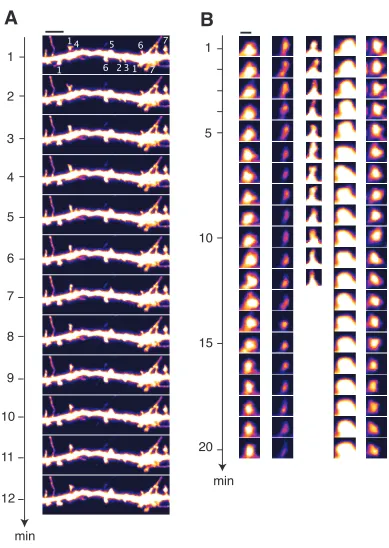
µm. (B) Time-lapse images of five individual spines showing subtle forms of spine motility. Scalebar = 1 µm. All images are acquired once every minute. Intensity of the cell-filling fluorophore EGFP is pseudo-colored with the “fire” look-up table in IMAGEJ.
2.1 Spine quantifiers in the literature
Following is a brief chronological list of methods and measures that have been used in the literature to respectively describe and quantify spines and their motility.
• >1960. Various: Calculated spine numbers and densities per unit dendrite length in different studies.
• 1970. A. Peters and I. R. Kaiserman-Abramov (1970): Classified spines into thin,
stubby, and mushroom or cup-shaped.
• 1992. K. M. Harris’ group (Harris et al., 1992): Pioneered the use of serial electron microscopy to analyze spines based on spine length (L), head diameter (dh), neck diameter (dn), and subcellular composition to classify spines into stubby (Type I), mushroom (Type II), and thin (Type III, see chapter 1 for details of classification, and also Harris, 1999; Sorra and Harris, 2000 for their discussion on the subcellular structure of spines).
• 1995. D. A. Rusakov and M. G. Stewart (1995): Proposed a scheme for
automatically determining dendritic and total spine length using 3D reconstructions.
• 1996. S. J. Smith’s group (Dailey and Smith, 1996): Computed filopodial lengths,
and presented time-lapse images. Categorized dynamics by counting the number of spines that were stable, that disappeared, that appeared, and that were transient.
• 1998. A. Matus’s group (Fischer et al., 1998): Computed spine length and “major”
individual spines as a function of time. Used the Mann-Whitney U test (for rank sum)
to statistically compare spine lengths in live versus fixed tissue.
• 1999. K. Svoboda’s group (Maletic-Savatic et al., 1999): In addition to quantifying
the number and density of synapses, computed instantaneous lengths (Lt), and used
successive (signed) length differences (Lt = Lt - Lt-1) as a measure of spine
dynamics.
• 1999. R. Yuste’s group (Dunaevsky et al., 1999): Proposed a motility index defined
as M = (accumulated area - smallest area)/average area. Used the Mann-Whitney U
test (for rank sum) to statistically compare values of the index before and after
treatment.
• 2000. A. Matus’s group (Fischer et al., 2000): Defined shape factor as S = 4*area/perimeter, and used it to look at the shape evolution of spine heads. With this
they characterized how far spine heads were from being spherical or circular. This
was done on a few individual spines.
• 2001. M. Sheng’s group (Sala et al., 2001): Characterized spine shape with length and
major width (largest width in a direction perpendicular to length). Plotted them
separately with respect to time and compared cumulative distributions over many
spines between neurons of two different ages (7 and 18 days in vitro).
• 2002. W. B. Lindquist’s group (Koh et al., 2002): Presented an automated method for
detecting spines, computing their morphological parameters and volumes, and
performing shape classification on them from both static and time lapse images. The
strength of this work is the development of an automatic detection and classification
For motility characterization, most investigators have looked at the time traces of various shape and size quantifiers for individual spines. Statistics have generally been applied only to spine numbers and densities. Large-scale statistical comparisons across many spines, and between more than two conditions, are challenging and have rarely been done. Changes in spine position have not been explicitly and rigorously quantified, and shape quantifiers used thus far in the literature have not been sophisticated. The only exceptions in the above cases have been the work of Dunaevsky et al., 1999, where they present a likely candidate for a unified motility measure10 and apply statistics on data from 15 spines to distinguish between “before” and “after” conditions, and Svoboda’s group, where they examine several thousand spines to study ongoing spine loss and gain. There is, however, ample scope for further development of motility quantification.
2.2 Unified scheme for characterizing motility – size,
position, timescale, and shape
We propose that a unified view of spine motility can be obtained by considering changes in four independent dimensions, namely – size, position, timescale, and shape (Fig. 2-2A). We quantify size by the area or volume, position by the center-of-mass, timescales by imaging spines at sampling rates ranging from seconds to days, and shape using elliptic Fourier functions (EFFs) (Fig. 2-2A). Both the use of center-of-mass to describe instantaneous spine position and the use of EFFs are novel techniques in the spine motility field. In theory, changes can occur to a structure along any one of these dimensions independently of the others. In experiments, changes occur in more than one
A. Preprocessing: live imaging to spine verification
Imaging, deconvolution, and registration. Time-lapse images of neurons overexpressing EGFP were acquired as z-stacks on an inverted LSM 510 Meta (Zeiss) microscope. Image stacks were 3D deconvolved in IMAGEJ (NIH, “Iterative Deconvolve 3D” plugin (Dougherty, 2005)) using a theoretical estimate of the 3D PSF (IMAGEJ, “Diffraction PSF 3D” plugin). No further filtering was performed. Stacks at all time-points were registered to the first stack. The z-projection (maximum) of the stack at each time-point was obtained, and from this, dendrites were straightened in IMAGEJ. The images at this stage are referred to as raw images in the text.
corrected for using appropriate noise thresholds as discussed below. The verified spines
were then rotated appropriately to achieve vertical orientation.
B. Acquisition protocol
Although spine dynamics have been studied separately at different timescales by
researchers, these different timescales have not been studied simultaneously, and
therefore, the relationship between changes at different scales is unknown. In order to
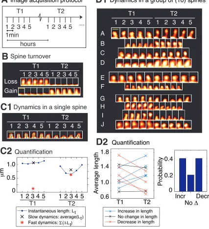
address this, we designed an image acquisition protocol (Fig. 2-3A) to acquire spine
images at two different timescales. Each acquisition “time-point” consisted of five
z-stacks imaged once every minute with a confocal microscope, representing the fast
timescale, and time-points themselves were acquired hours apart, representing the slow
timescale (Fig. 2-3A).
C. Size, position, and shape
After preprocessing the images, selecting and verifying spines, we not only
monitored spine loss and gain (Fig. 2-3B), but also computed several spine quantifiers
(covering the three dimensions of size, position, and shape) like length, area,
center-of-mass, spine type, major axis, head diameter (minor axis) for each spine at each instant
using custom codes in MATLAB. The use of EFFs for shape quantification is described
in section F below. For these above calculations, thresholded images were used so that
the confounding effects of EGFP intensity distributions on estimating spine morphology
were minimized. Thresholds were automatically determined using a modified Otsu’s
method. The instantaneous centerline (“backbone”) of a spine was estimated from the
thresholded image by successively computing the midpoint of all non-zero pixels in each
spine length (Lt) was calculated as the arc length of this centerline. The instantaneous center-of-mass was calculated as x(t) = (xc(t),yc(t)) = (i=1N(t)
xi(t)/N(t), i=1N(t)yi(t)/N(t)), where (xi(t), yi(t)) are the positions of all non-zero pixels in the thresholded spine image at time t and N(t) is the total number of non-zero pixels at that time.
D. Two timescales in each quantifier
We then characterized fast and slow dynamics of each spine morphological
quantifier. Slow timescale dynamics were evaluated for each quantifier (for instance
spine length) was calculated as the average value of that quantifier (average length) over
the five samples within each time-point. Fast timescale dynamics in a quantifier was
computed as the sum over the five samples of the absolute value of the successive
differences in the quantifier. For instance, length motility at each time-point was
calculated as t=25
(Lt-Lt-1), and center-of-mass motility within each time-point is calculated as t=25 |x(t) – x(t-1)|. Fig. 2-3, C1 and C2 show the fast and slow length dynamics in a single spine, referred to as length motility and average length, respectively.
E. Comparing groups of spines
The diversity in spine dynamics in control neurons, evident even in nearby spines
on the same dendrite, makes the reliable detection of experimental effects challenging.
We found that comparing the probabilities of change between treatment and control was
a robust method for detecting treatment effects that are not revealed by comparing
population means. To this end, for instance, in a group of 10 control spines (Fig. 2-3D1),
the probabilities of change in average length (slow length dynamics) are calculated as the
fractions of spines that show an increase, no change, or decrease (Fig. 2-3D2) in length
from a control neuron that show spine loss (top image) and gain (bottom image), i.e., spine turnover – the most extreme form of spine morphological change. (C) Characterizing morphological dynamics in a single spine at the two timescales, with spine length as the example quantifier. (C1) Time-lapse images of an example spine from a control neuron acquired at the two time-points. The automated centerline generated to compute spine length at each instant is indicated as a one-pixel-wide black curve (see Methods). (C2) Instantaneous length (Lt, blue circles); slow length dynamics, or average
length (average (Lt) within each time-point, black cross); and fast length dynamics, or
length motility (|Lt| within each time-point, red asterisk). The spine in (C1) shows a
decrease in average length (slow timescale), but an increase in length motility (fast timescale). (D) Characterizing dynamics in a group of spines, with average length (slow length dynamics) as the example quantifier. (D1) Time-lapse images of 10 example spines A-J from a control neuron, in which four spines A-D show an increase in average length, two spines E-F show no significant change, and four spines G-J show a decrease, with respect to T1. To determine the magnitude of change in the value of a quantifier that can be considered significant, we have experimentally measured noise thresholds that estimate the extent of change that can occur due to various sources of noise (see Fig. 2-5). (D2) (Left panel) Average lengths of spines A-J at the two time-points T1 and T2. (Right panel) Probabilities of change in the average length of spines A-J at time-point T2 with respect to time-point T1, calculated as fractions of spines. In the rest of the paper, dynamics in spine groups are characterized with probabilities, and comparisons between treatment and control are made with respect to these probabilities. All spines in this figure are from control neurons; T1 was the baseline time-point taken before control treatment, and T2 was the time-point 75 minutes after it. Scalebars in yellow = 1 µm.
F. Noise sources – correcting for them or estimating their contributions
Confocal microscopy (see Yuste et al., 2000) is an established tool for
high-resolution fluorescent imaging (Fine et al., 1988; Michalet et al., 2003; White et al.,
1987). Fluorescence markers have been used for over half a century now, and the ability
(see Lippincott-Schwartz and Patterson, 2003; Miyawaki et al., 2003 for reviews).
Further, GFP-based fluorescence has been used specifically for spine motility studies in
hippocampal tissue since 1998 (Fischer et al., 1998). Nevertheless, specific to spine
motility studies, there is potential data contamination by various sources of noise and this
needs to be addressed. Noise effects are especially pertinent for our studies given the
quantifiers we define and the desire to detect relatively subtle effects. We list below the
sources of noise and discuss the means we have implemented to correct for them.
Lens-induced blurring. Any image obtained through a set of lenses results in a blurred image due to diffraction effects. This increases the sensitivity to noise and
decreases the effective resolution in all three spatial directions. To correct for this, 3D
deconvolution was performed during preprocessing, as described above.
Spurious movement. As we are interested in the fine movements of small structures in neural tissue, any extraneous, or large-scale, movement of the either the dish
itself, or of dendritic processes, is a source of error. We minimized dish movement during
imaging by securing the dish on the microscope stage with fixtures. Dish movement and
movement of dendritic processes between time-points (extraspinal movements) was
corrected for to a large extent post-acquisition with 3D image registration and verification
as described above. The confounding effects of any residual extra-spinal movement on
“real” spine motility were corrected for using an estimated noise threshold that included
spurious movement (Fig. 2-4).
GFP diffusion. Since the signal (image) is dependent on the presence of GFP in various parts of the cell, one source of noise is the spontaneous change in the distribution
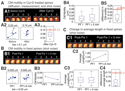
interested in monitoring. We expect that after about 12 hours of viral expression (which is the duration of viral expression in our protocol), macroscopic GFP distributions are stable in the cells. However, ongoing diffusion within tiny compartments like spines can confound quantification, particularly the estimation of fast dynamics. We estimated the contribution of diffusion and residual extra-spinal movement to motility by imaging spines before and after the application of cytochalasin D (Cyt-D), a drug that interferes
with actin polymerization and is known to block spine dynamics (Fischer et al., 1998)
(Fig. 2-4A). Therefore, any dynamics observed post-Cyt-D provides a reliable estimate of
the noise in the quantification of motility.
Spurious change in quantifier value. In order to estimate probabilities of change (as described in subsection E above), we need to know reliably whether or not there was a change. For this, we must estimate the magnitude of change that can occur due to noise. The most likely contributor to spurious change is shot noise. Shot noise occurs when electrons are spontaneously emitted by the photomultiplier tube (PMT) in the absence of real excitation.12 Thermal effects are the most common cause of shot noise. To estimate the contribution of shot noise alone, we imaged fixed tissue obtained after the fixation and immunostaining of GFP-expressing neurons. Two time-points were taken post-fixation and various quantifiers of fast and slow dynamics were computed at each time-point. The difference between the values of a quantifier at the two time-points for every spine was calculated and the distributions plotted. The 95-percentile value of this distribution was chosen as a reasonable estimate of spurious change in that quantifier.
Fig. 4B estimates the noise threshold for change in center-of-mass motility, and Fig.
2-4C, in length motility.
Photobleaching. Finally, photobleaching is a critical issue in fluorescent imaging
(see Lippincott-Schwartz et al., 2003). Fluorescent probes work by absorbing light at a
particular frequency and emitting light at a lower frequency (Stokes shift, (Hibbs, 2000)).
This happens when electrons in the dye molecule are excited to a higher state upon
absorption of the excitation spectrum and then emit lower frequency photons as they
return to their ground state. Not all the light absorbed by a dye molecule is used to
produce fluorescence – there are concomitant heat losses. More importantly, electrons do
not always return to the ground state from the excited state. There is a small probability
(~0.03) that the energy is used to create chemical reactions which can affect the
properties of the dye and render it dull and unable to fluoresce. This is called
photobleaching. Although the probability of this interstate conversion is very low, the
fluorophore can remain in this unusable state for a long time. Thus there can be a loss of
signal. Especially, as we are interested in morphology determination over time, loss of
the usable fluorophore due to bleaching can be indistinguishable from the actual
shrinkage of a spine. We minimized photobleaching by using low-intensity laser light
(0.5%). Further, GFP has a very tight crystal structure with the residues responsible for
fluorescing being buried deep in an -helix surrounded by -barrels (Hibbs, 2000;
Sullivan and Kay, 1999). This structure renders the fluorophore fairly resistant to
(0.12 µm) was chosen as the noise threshold. (B) Estimate of spurious change in
center-of-mass motility (predominantly due to shot noise, see text for details). (B1) Time-lapse
images of a representative spine at two time-points that are both obtained after fixing
neurons expressing EGFP and immunostaining them for EGFP. (B2) Loci of the
instantaneous center-of-mass positions of the example spine (B1) within each of the two
time-points (left and right panels, respectively). The numbers in microns indicate total
movement at that time-point. The difference between these two values is small, as
expected. (B3) Center-of-mass motility of the example spine (B1) at the two time-points.
(B4) Box plots showing the distributions of center-of-mass motility values at the two
time-points after fixation (n=128 spines). (B5) Box plot of the distribution of the absolute
difference between the center-of-mass motility values measured at the two time-points.
The 95-percentile value of this distribution (0.039 µm) noise was chosen as the noise
threshold for change in center-of-mass motility. (C) Estimate of spurious change in
average length of spines. (C1) Time-lapse images of the example spine shown in (B1)
with the instantaneous centerlines. (C2) Average length of the spine at the two
time-points. (C3) Box plots showing the distributions of spine average length values at the two
time-points after fixation (n=128 spines). (C4) Box plot of the distribution of the absolute
difference between average length values measured at the two time-points. The
95-percentile value of this distribution (0.14 µm) noise was chosen as the noise threshold for
change in average length.
G. Advanced shape quantification with EFFs
Determining EFFs from spine image. When Fourier series (Oppenheim et al.,
1999) are obtained from the parameterized x and y coordinates of a closed contour, the
resulting coefficients are called elliptic Fourier functions (EFFs (Lestrel, 1997; Mysore,
1999; Zahn and Roskies, 1972)). A great advantage of using EFFs is the ability to
achieve smooth reconstruction of sampled, polygonal boundaries and to summarize shape
with a sparse approximation. In our case, the object whose shape we wish to summarize
parameterized by arc length along the boundary. If the spatial coordinates of a contour
pixel i are (xi,yi), then we can collect all the pixel coordinates as walk along the contour,
having started at pixel i0 and returning to it. The collection of coordinates is now an
ordered set, ordered by the parameter arc length, s. The contour can now be described
with two piece-wise continuous, parameterized functions: xi = ui(s) and yi = vi(s), i=1 to
N. The top-left and top-right panels of each subfigure in Figs. 2-5 (and 2-6) show,
respectively, in cyan, ui(s) and vi(s) for the spine shown in the bottom-right panel. Fourier
series can now be fitted to xi = ui(s) and yi = vi(s) and the Fourier coefficients (or EFFs)
obtained. For each curve ui and vi, there are ~N+1 coefficients, corresponding to
frequencies ranging from zero to the maximum spatial frequency in the curve.
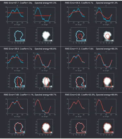
Using EFFs for spine-shape characterization. With these coefficients,
reconstructions with increasingly better accuracies are achieved by using progressively
more and more coefficients during the reconstruction process (shown going from Fig.
2-5A to F and Fig. 2-6A to F). Once reconstructed versions of xi and yi are obtained, they
can be plotted separately (in red, in the top two panels of each sub-figure), or together,
showing the reconstructed contour in 2-D (shown in red in the bottom two panels of each
sub-figure). If just the first EFF is used, then the resulting 2-D reconstruction will
correspond simply to the mean; on the 2-D plane it is a point corresponding to the center
of mass (bottom panels in Fig. 2-5A and Fig. 2-6A). As the number of coefficients used
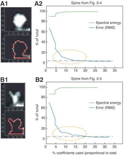
is increased, the reconstruction begins to resemble the original contour more. A plot of
the error in reconstruction (blue line, root mean squared error between the original
contour and the reconstructed contour calculated point by point) as a function of the
The horizontal, black dash-dashed line is a threshold for acceptable error (set arbitrarily
at 4%). The x-axis is the percentage of coefficients used, and the frequencies included
increase with the percentage of coefficients. The yellow, dashed ellipses show differences
in the evolution of error, with corresponding differences in the spectral energy (green
line). EFFs can be used to summarize shape in many ways. One is by comparing the
evolution of the error and energy curves. Another is by using a norm to quantify the
difference between the coefficients-vector. A third is to ask what frequencies are
represented if only those coefficients which contribute maximally to 90% of the spectral
energy, or which result in a 10% error in reconstruction. Thus, either multivariate or
univariate EFF summaries can be used to distinguish differences between spine shape
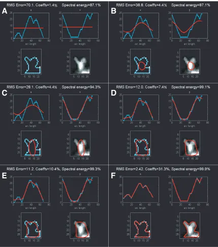
over time, or across spines. Here, the spine in Fig. 2-6 has spinules (tiny projections from
spine heads), which are represented in higher frequencies. In comparison with the spine
in Fig. 2-5, this is evident if we compare the error profiles (Fig. 2-7) – the error reaches
the threshold at a higher frequency (greater % of coefficients used) because of an earlier
plateau. Such differences can be systematically characterized and subtle changes in spine
shape detected by understanding the patterns corresponding to different spine shapes.
Noise estimates can be obtained as they have been for other quantifiers thereby
separating real shape change from the spurious. We have custom code that automatically
A
B
C
D
E
F
% %
% %
Figure 2-5. Summarizing spine shape with EFFs – example 1.
A
B
C
D
E
F
%
% %
%
Figure 2-6. Summarizing spine shape with EFFs – example 2.
and then these distributions are compared between treatment and control. We also
describe a sophisticated spine shape characterization scheme that can detect shape
differences. We are thus able to reliably measure gross as well as subtle spine
Chapter 3.
Regulation of spine dynamics
and synaptic function by N-cadherin
3.1 Introduction
In the face of stable memories, neuronal synapses are in a constant state of flux
both biochemically (Inoue and Okabe, 2003; Malinow and Malenka, 2002) and
structurally (Dailey and Smith, 1996; Dunaevsky et al., 2001; Holtmaat et al., 2005;
Knott et al., 2006; Majewska and Sur, 2003; Trachtenberg et al., 2002; Zuo et al., 2005).
Dendritic spines, the post-synaptic sites of most excitatory synapses, show a wide range
of morphological changes mediated by the dynamics of the underlying actin cytoskeleton
(Fischer et al., 1998). These changes can be described along two general dimensions: (1)
timescale – ranging from seconds (Fischer et al., 1998; Korkotian and Segal, 2001) to
days (Grutzendler et al., 2002; Holtmaat et al., 2006; Holtmaat et al., 2005; Mizrahi and
Katz, 2003; Trachtenberg et al., 2002), and (2) degree – ranging from subtle changes such
as in the ruffling of membranes (Fischer et al., 2000; Korkotian and Segal, 2001) to the
appearance and disappearance of spines (Engert and Bonhoeffer, 1999; Holtmaat et al.,
2006; Maletic-Savatic, 1999; Nagerl et al., 2004; Trachtenberg et al., 2002). The faster
and more subtle forms of motility (e.g., head morphing and changes in spine neck size)
are thought to regulate calcium compartmentalization (Korkotian and Segal, 2001;
Majewska et al., 2000) and protein scaffolding (Dillon and Goda, 2005; Halpain, 2000)
and thereby biochemical signaling at the synapse, while the slower and more extreme
thought to mediate synaptic and architectural plasticity (Holtmaat et al., 2006; Lang et al.,
2004; Matsuzaki et al., 2004; Okamoto et al., 2004; Trachtenberg et al., 2002; Zhou et al.,
2004; Zito et al., 2004). Though the contributions of individual molecules to spine
morphology have been studied in detail (see Lamprecht and LeDoux, 2004; Tada and
Sheng, 2006 for reviews), little is known about whether ongoing structural dynamics
provide any information about future changes in the network synaptic structure.
As discussed above, even in control neurons, spines display a wide variety of
morphological dynamics. Comparing these ongoing dynamics in control neurons to the
effects of a treatment capable of altering them can highlight associations between various
forms of spine motility and reveal their regulation. Particularly, the relationships, if any,
between changes at different timescales, and any predictive associations therein, can be
studied via such comparisons to a stochastic baseline. Towards this end, we hypothesized
that interfering with the structural constraints of a synapse (Berardi et al., 2004; Oray et
al., 2004), by disrupting synaptic adhesion molecules involved in the maintenance of
synaptic structure (Abe et al., 2004; Togashi et al., 2002), would be a direct approach. In
particular, we decided to disrupt N-cadherin, a Ca2+-dependent, homophilic, synaptic
adhesion molecule (Fannon and Colman, 1996; Redies, 2000; Salinas and Price, 2005;
Shimoyama et al., 2000; Takeichi, 1991; Takeichi and Abe, 2005; Uchida, 1996;
Wheelock and Johnson, 2003). N-cadherin is implicated in synapse assembly (Benson
and Tanaka, 1998; Boggon et al., 2002; Hirano et al., 2003; Jontes et al., 2004; Shapiro,
1999; Togashi et al., 2002), in the formation of synaptic circuits (Redies et al., 1992;
Takeichi et al., 1997), and is known to be involved in synaptic plasticity (Benson and
1998) Particularly, the disruption of N-cadherin by the overexpression of a
dominant-negative form for 3 days leads to significant changes in spine morphology and synaptic
organization (Togashi et al., 2002). Further, the disruption of N-catenin, a molecule
involved in cadherin-mediated adhesion, by gene knockout results in spines that are
abnormally motile (Abe et al., 2004). Additionally, N-cadherin is linked to the actin
cytoskeleton, the physical effector of motility (Fischer et al., 1998), via intermediary
proteins (Hirano, 1992; Ozawa, 1990a), and this linkage is key to its adhesive function
(Braga, 2002; Braga, 1997; Fukata and Kaibuchi, 2001; Nagafuchi, 1994). The above
evidence suggests that N-cadherin-mediated adhesion can regulate synaptic structure and
is therefore a good candidate for the study of spine dynamics. However, exactly what the
effects of directly disrupting N-cadherin are on spine dynamics, in mature synapses, and
in response to a short-term disruption (as opposed to several days of inhibition), are all
unknown.
With this background, we proceed to systematically characterize spine dynamics
in the context of direct and acute N-cadherin disruption at mature hippocampal synapses.
In addition to investigating the structural consequences, we ask what signaling
mechanisms downstream of N-cadherin may be involved in mediating the observed
effects.
3.2 Methods
A. Cell culture and infection
Dissociated hippocampal neurons were prepared from post-natal day 2
Sprague-Dawley rat pups and plated at a density of 310-460/mm2
, as described in Aakalu et al.,
neurons were infected with Sindbis EGFP (in spine dynamics experiments) or Sindbis
-catenin-GFP (in -catenin dynamics experiments) for 20 minutes and, after a wash,
returned to filtered, conditioned growth medium and placed in a 37°C incubator for 10 hours. The growth medium was replaced by HBS (HEPES buffered saline) and allowed
to equilibrate for 2 hrs in a 37°C, 5% CO2 incubator prior to image acquisition.
B. N-cadherin disruption
The 5-mer peptide AHAVD (HAV) is known to interfere with the function of
N-cadherin (Chuah et al., 1991; Tang et al., 1998), and its efficacy is enhanced by low
extra-cellular Ca2+
concentrations (e.g., less than 2 mM) (Tang et al., 1998). We acutely
disrupted N-cadherin with a 10 min pulse application of 2 µM AHAVD (“HAV” peptide) in a zero Ca2+
medium containing 1 mM EGTA at 37°C, followed by a wash and replacement of HBS. As control we used a scrambled 5-mer peptide AADHV (“SCR”) at
the same concentration. The treatment (or control) was applied after acquisition of
baseline images, and at the appropriate time-points further image stacks were acquired.
C. Live imaging
All imaging was performed on an inverted LSM 510 Meta (Zeiss) microscope.
Neuronal images were acquired as z-stacks with an oil-immersion objective (Plan
Apochromat 63x, N.A. 1.4, Zeiss) at a zoom of 2. The x-y-z resolution was
0.07x0.07x0.37 µm/pixel. Except for the brief periods during image acquisition, neurons were maintained with HBS at 37°C, 5% CO2 throughout the experiment.
D. Analysis
Preprocessing and analysis was performed as described in detail in chapter 2.
visualization in the figures, spine images were median (2x2) and mean (2x2) filtered.
These images were then pseudo-colored for display so that EGFP intensity in spines was
represented with the hot colormap in MATLAB in which black corresponds to an
intensity of 0, white to 255, and various shades of red and yellow to intermediate
intensity values. Data for Figs. 3-1 to 3-4 (relating to the investigation of spine dynamics)
are from 690 spines (HAV) and 803 spines (SCR) across three experiments. These spines
were segregated randomly into n=14 and n=16, groups respectively, each containing 50
spines. This allowed us a sample size large enough to estimate probabilities but not so
large that we would lose statistical power for comparisons. Probabilities of change in a
quantifier were estimated for each group of 50 spines and then these distributions were
compared between treatment and control. Data for Fig. 3-5 (for -catenin dynamics
experiments) are from 483 spines (HAV) and 465 spines (SCR).
E. Statistical comparisons
All data are plotted as mean ± SEM. T-tests were used to evaluate the differences
between various sampled distributions, and “*” represents significance at p<0.05 for
unpaired comparisons (2 groups). Multiple t-tests (>2 groups) were performed where
necessary in all figures after applying a correction for multiple comparisons. Many
standard correction schemes exist and, here, we tried two different ones – a conservative
Bonferroni approach, and a less conservative, but equally well-accepted, scheme of
estimating the false discovery rate (FDR) (Genovese et al., 2002) with an acceptable FDR
of 5%. With both approaches, the comparisons that came out as significant were
identical. “*” represents significance at p<0.05 after correction. Comparisons that are not
F. Electrophysiology
Whole-cell patch-clamp recordings were performed with an Axopatch 200B
amplifier on cultured hippocampal neurons bathed in HBS containing in 1 µM TTX and
20 µM bicuculline. Whole-cell pipettes (with a resistance of 2.5-5 M) were filled with
an internal solution of pH 7.2 containing in mM: 100 cesium gluconate, 0.2 EGTA, 5
MgCl2, 2 ATP, 0.3 GTP, 40 HEPES. Neurons with pyramidal-like morphology were
voltage-clamped at –70 mV, and series resistance was left uncompensated. Membrane
parameters and series resistance were monitored at the beginning and end of each
recording and only cells with less than 20% change in series resistance were included for
analysis. Mini analysis software (Synaptosoft) was used to manually detect minis. The
data are from 8-9 neurons in each condition, from 7 independent experiments paired for
HAV and SCR treatments.
G. Immunoprecipitation
After the appropriate treatments (HAV or SCR), neuronal cell lysates were
precleared overnight with rabbit IgG. They were then incubated for 4 hours with either
rabbit anti--catenin (Zymed) or rabbit anti-IgG, and with 40 uL protein-G beads
(SIGMA). The beads were spun down, separated from the supernatant, boiled, and then
loaded onto 7.5% SDS-PA gels. SDS-PAGE was performed at 80 mV for 4 hours.
Proteins were transferred overnight to PVDF membranes, and then probed for several
proteins successively, with intermediate acid-washing steps when necessary. The data are
H. Immunofluorescence
Sample preparation. Neurons were treated with HAV or SCR peptides for 10
minutes, then allowed to recover in conditioned growth medium at 37°C for 30 min, 75
min, or 150 min. They were then antibody live-labeled by first rinsing with ice-cold zero
Ca2+ HBS containing 1 mM EGTA and incubated on ice for 30 min in mouse
anti-surface-N-cadherin antibody (produced and purified in the lab by Dr. Chin-Yin Tai, 1:50
dilution in HBS/0 Ca2+/EGTA). After rinsing, they were fixed with 4% PFA/4%
sucrose/PBS-MC on ice for 10 min, permeabilized with 0.1% Triton-X-100/2% BSA
/PBS-MC for 10 min, rinsed, blocked in 2% BSA for 20 min, and incubated with rabbit
anti-beta-catenin (1:500, Zymed) primary antibody for an hour. Neurons were then
incubated in a mixture of goat anti-mouse Alexa 488 (1:1000) and goat anti-rabbit Alexa
546 (1:1000) secondary antibodies for an hour. Cells were lightly fixed again (2%
PFA/2% sucrose/PBS-MC) for 5 min. Zenon Alexa Fluor 633 Mouse IgG2a (Invitrogen)
was then coupled to mouse anti-bassoon primary antibody following the suggested
protocol and cells were incubated in this conjugate for 30 min at room temperature.
Prolong gold anti-fade reagent (Invitrogen) was applied to preserve fluorescence for
longer periods, and neurons were sealed between glass-slides to ready them for imaging.
Imaging post-fixation. Imaging was done on an inverted LSM 510 Meta (Zeiss)
microscope using an oil-immersion objective (Plan Apochromat 63x, N.A. 1.4, Zeiss) at a
zoom of 1. Pyramidal neurons were selected based on their surface N-cadherin staining
(Benson and Tanaka, 1998), and image z-stacks were acquired in three colors (excitation
laser lines– 488 nm, 546 nm, and 633 nm) using multi-track imaging with appropriate
filter sets (multi-track imaging minimizes bleed-through across channels, and when we
parameters used). Appropriate filter sets were used for collection. For analysis, dendrites
were straightened, 3D deconvolved, and watershed filtered in IMAGEJ to improve
puncta separation. These images were then analyzed using custom code written in
MATLAB to determine puncta sizes, volumes, and intensities in 3D. Fig. 7 is based on
data from 32-46 dendrites for each treatment, at each of the time-points.
I. L-cells aggregation assay
L-cells were transfected with N-cadherin using Lipofectamine 2000 (Invitrogen)
and a gentamycin-resistant stable line was created after a month of passaging. L-cells
were plated onto 10 cm dishes in DMEM complete and allowed to reach confluency for
two to three days. They were then trypsinized, counted, and approximately 500 µL of cell suspension (at 0.95-1.07x10⁶
cells/100 µL) was used for each of three treatments – 2 µM HAV, or 2 µM SCR, or HBS. After a 10 min incubation at 37°C, they were rinsed with and suspended in DMEM complete. Immediately, 10 µL of cell suspension from each sample was mounted onto slides. This represented time t=0. The samples were all placed
in a 37°C shaker at 500 rpm. At each of t=30, 75, 150, and 180 min, cell suspensions were plated onto slides as before and imaged in DIC on an inverted LSM 510 Meta
(Zeiss) microscope using an air objective (10x Plan-Neofluar, N. A. 0.3, Zeiss) at a zoom
of 0.7. The extent of aggregation was quantified (Nguyen and Sudhof, 1997) as N0/Nt,
where Nt was the number of cells not in aggregates at each t. Data are from three
3.3 Results: fast and slow spine dynamics are precursors
of spine loss
To study different forms of structural dynamics in dendritic spines and their
relationships to one another, we conducted high-resolution time-lapse confocal imaging
of hippocampal dendrites and spines before and after the acute disruption of the Ca2+
-dependent cell-adhesion molecule, N-cadherin. We hypothesized that interfering with
synaptic adhesion (Abe et al., 2004; Togashi et al., 2002) would lead to changes in spine
dynamics. This allowed us to examine whether fast spine dynamics, observed within
minutes, might predict morphological changes observed over the time course of hours. To
address this, we acquired images of spines at two different timescales as described in
chapter 2 (Fig. 2-4): the fast timescale was over minutes, and the slow over hours. We
have determined the contribution of noise (diffusion, extra-spinal movement, and shot
noise) to our measurements (Fig. 2-5) and established that we can detect subtle changes
in spine morphological quantifiers above noise.
A. More spines are motile after N-cadherin disruption
As N-cadherin is involved in the structural stability of synapses (Goda, 2002;
Takeichi and Abe, 2005), we asked whether disrupting N-cadherin-mediated adhesion
would lead to increased spine movement. We perturbed surface N-cadherin with the
function-interfering HAV peptide (AHAVD, Chuah et al., 1991; Tang et al., 1998) and
then monitored the fast and slow dynamics of individual spines at 75 and 180 min after
this treatment. We first examined rapid changes by analyzing the fast center-of-mass
dynamics (center-of-mass motility) of individual spines (Fig. 3-1). This measure of
motility is influenced by lateral and protrusive spine movements and is a general
increase in center-of-mass motility at 75 min than in control peptide-treated cells
(scrambled AADHV peptide, SCR, Fig. 3-1C). Surprisingly, this effect was no longer
observed at 180 min. There was no significant difference at baseline between the
center-of-mass motility distributions of HAV and SCR spines, and additionally, length motility
and area motility were unaffected by cadherin disruption (data not shown). To check whether the effects on center-of-mass motility observed at 75 min could be due to a
preferential effect of HAV on GFP diffusion, we performed fluorescence recovery after
photobleaching (FRAP) experiments on GFP-expressing neurons at 75 min after the
application of either HAV or SCR (Fig. 3-1D). FRAP experiments help estimate rates of
diffusion of a fluorophore (in this case GFP). Since the recovery rates of GFP after HAV
or SCR treatments are indistinguishable (Fig. 3-1D2), we can rule out any confounding
effects of HAV on GFP diffusion. These results show a preferential regulation of fast
to center the locus at the origin). The large filled circle represents the position of the
spine at the first minute within that time-point. The locus in each panel gives a visual
indication of the extent to which the spine is motile. The center-of-mass motility value
(net movement) of the spine within a time-point is indicated above the panel. The
scalebar = 0.1 µm and applies to all panels. (B2) Center-of-mass motility of the example
spines is plotted normalized to baseline. There was no significant difference at the
baseline time-point in the center-of-mass motility values between the HAV- and
SCR-treated spine populations. (C) Summary data showing the probabilities of increase
(pIncrease), no change (pNochange), and decrease (pDecrease) in the center-of-mass
motility of all persistent spines. The motility value of a spine at each time-point was
compared to that at baseline to determine the nature of change. Probabilities of change
were estimated from groups of 50 spines (see Methods). Data in this and subsequent
figures are based on approximately 1500 spines from HAV- and SCR-treated cells. (D)
Fluorescence recovery after photobleaching (FRAP) at 75 min after either HAV or SCR
treatment. (D1) Time-lapse images of representative spines from HAV- and SCR- treated
cells showing FRAP. (D2) Individual FRAP curves from four spines for each of the two
treatments (red dots – HAV, blue dots – SCR), along with the average FRAP curves for
each treatment (thick solid lines). The average curves for HAV and SCR spines were
nearly identical. Scalebar = 1µm.
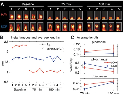
B. More spines shrink in length after N-cadherin disruption
We next examined if N-cadherin disruption had an effect on slow spine dynamics
(Fig. 3-2). We found that more spines showed a reduction in slow length dynamics
(average length) 75 min after N-cadherin disruption (Fig. 3-2C). Again, as with
center-of-mass motility, this effect was not observed 180 min post-treatment (Fig. 3-2C), and
there was no difference between the average length distributions of HAV- and
SCR-treated spines (data not shown). These data show that N-cadherin disruption
preferentially produces a decrease in average length (slow timescale) and an increase in
Figure

Related documents