Faculty of Engineering Technology
Department of Mechanical Engineering
Chair of Production technology
CONFIDENTIAL
A Rapid Prototyping system for the
Hot-Wire Cutting process
Master Thesis
A Rapid Prototyping system for the
Hot-Wire Cutting process
Master’s Thesis - Mechanical Engineering
by
J.H. VAN RAVENHORST
Student number: s0010979
Submitted in partial fulfillment of the requirements
for the degree of Master of Science
Examination committee:
Prof. Dr. Ir. R. Akkerman Supervisor, University of Twente Ing. C. van Driel Supervisor, 3EL-Company bv Ir. G. van Ouwerkerk University of Twente
Ing. A. de Smit Delft University of Technology Ir. H. Tragter University of Twente
Institute of education: Master Project location: Chair of Production Technology 3EL-Company bv
Department of Mechanical Engineering Enschede, The Netherlands Faculty of Engineering Technology
University of Twente Enschede, The Netherlands
Abstract
Samenvatting
Acknowledgements
First of all, I would like show my gratitude to my parents for their unconditional support of their eldest son who embarked at this rather technical study at the University of Twente, bearing the name of ‘Mechanical Engineering’.
The master project activities were located at 3EL-Company bv in Enschede, The Netherlands. I would like to thank my supervisor Cock van Driel from 3EL-Company for his advice and shared knowledge about both hot-wire cutting and its applications. I also want to thank Annelies van Driel who compensated for the technical and theoretical neuroses of the men around her in the company.
From the University of Twente, also located in Enschede, I would like to thank my supervisor Professor Remko Akkerman who, in spite of his enormous amount of activities, was always willing to find time and share ideas. Appreciation is also there for my fellow-students and staff at the chair of Production Technology who attended the meetings during the master project, leading to helpful discussions about various subjects.
Quite some time was spent to make crucial decisions and it was Hans Tragter who helped me convince in choosing direct slicing over tessellated slicing. This was not until later on in the process, where its advantages became more clear, that I learned to appreciated it. I also would like to thank his students for their time and thought of several slicing-related problems.
The conceptual design of the Skymobil body as used throughout this work was made available by G¨otz Steudel, a retired engineer from Germany. It is part of the Skymobil project involving the development of a flying car, primarily involving an EPS-carbon sandwich construction. His inspiration was most welcome.
List of Symbols and
Abbreviations
The following lists include the most important nomenclature used throughout this work. The page numbers denote the first location of appearance. Unlisted nomen-clature receives its descriptions from the context and can have multiple meanings, depending on the location of appearance.
Symbols
arc length ratio, page 41
∗ minimum arc length ratio for a single layer, page 42
min minimum allowed arc length ratio, page 42
δ cusp height or maximum normal deviation, page 27 m
error in layer plane, page 32 m
ˆ
I ‘unit change’-based thickness list index, page 43
κ curvature of a curve, page 30 m−1
κn normal curvature of a surface, page 30 m−1
κn,1 maximum principal curvature, page 31 m−1
κn,2 minimum principal curvature, page 31 m−1 B binormal vector, page 77
D second fundamental matrix, page 80 G first fundamental matrix, page 79
ρ radius of curvature, page 29 m
σ standard deviation, page 110
θ wire angle, page 39
θ∗ maximum wire angle for a single layer, page 39
˜
I κn-based thickness list index, page 43
~c unit correspondence vector, page 40
~
d unit direction vector which, together with ~nS, defines plane P,
page 29
~e1 maximum principal curvature direction, page 31
~e2 minimum principal curvature direction, page 31
~ez build direction, page 13
~n nominal unit surface normal vector, page 28
b (subscript) denotes the base of a layer, page 20 t (subscript) denotes the top of a layer, page 20
C parametric curve, page 20
e actual normal deviation, page 30 m
e∗ maximum absolute actual normal deviation for a single layer,
page 40 m
I final thickness list index, page 43
R ruled parametric surface, page 20
S nominal parametric surface, page 27
s arc length, page 77 m
T layer thickness, page 43 m
t layer thickness estimation, page 29 m
t∗ critical (smallest) layer thickness estimation, page 30 m
u parameter of a parametric curve or first parameter of a paramet-ric surface, page 79
v second parameter of a parametric surface, page 79 Abbreviations
API application programming interface, page 46 CAD computer-aided design, page 12
EDM electrical discharge machining, page 17 FEM finite element method, page 19
HWC hot-wire cutting, page 10 KWC kerf width correction, page 26 LM layered manufacturing, page 12
LMT layered manufacturing technologies, page 12 NURBS non-uniform rational B-spline, page 19
NVP normal vertical plane - a plane spanned by~nS and ~ez, page 29
PG photogrammetry, page 108 RHR right hand rule, page 49 RMS root mean square, page 110 RP rapid prototyping, page 12 SE Solid Edge, page 46
SFF solid freeform fabrication, page 12 STL stereo lithography (file format), page 18 SW Solidworks, page 46
Contents
Abstract 1
Samenvatting 2
Acknowledgements 3
List of Symbols and Abbreviations 4
3.5.4 Error analysis . . . 40
C Application iteration flow charts 82 C.1 Flow chart legend . . . 82
D Application algorithm flow charts 89
D.1 Iteration flow charts (continued) . . . 89
D.2 Correspondence solving flow charts . . . 93
D.3 Actual error flow charts . . . 100
E Edge topology traversal 101 E.1 Edge assignment for correspondence solving . . . 101
E.2 Topology traversal . . . 102
F Demonstrator slicing results 104 G Accuracy analysis 108 G.1 Introduction to Photogrammetry . . . 108
G.2 Photogrammetry measurement setup . . . 109
G.3 Photogrammetry accuracy . . . 111
G.4 Single layer accuracy analysis . . . 114
G.5 Layered model accuracy analysis . . . 115
Chapter 1
Introduction
In this chapter, hot-wire cutting and the rapid prototyping process are introduced. Both techniques are tightly connected. Rapid prototyping techniques are essential for advanced use of hot-wire cutting, as will become clear in this chapter. Def-initions used in the rapid prototyping area are presented as far as applicable to this work. Next, the purpose of the overall programme is described as well as the problem being investigated in the master project. Finally, the outline for the rest of this work is given.
1.1
Introduction to hot-wire cutting
The ‘hot-wire cutting’ (HWC) process is used to cut foams made of polystyrene or other thermoplastic materials. HWC was partly developed in the area of model airplane building. Currently, it is used for various applications. Examples are the production of models and molds for the wind turbine blade industry and ship hull production. Other applications are the production of display signage, free form architecture, skatepark shaping and many others. It is also used as a preprocessing step for milling.
HWC makes use of a current that is fed through a wire which heats up as a consequence, reaching a temperature that is sufficiently high to vaporize and melt the foam. Ideally, the foam is vaporized just ahead of the advancing wire instead of being touched by it. The most common application is using the wire in a straight line while subjected to an actively controlled tension, allowing it to make so called ‘ruled surfaces’. See also section 2.5.1 for its definition. The principle of HWC is shown in figure 1.1 with a four-axis ‘computer numerical controlled’ (CNC) HWC machine.
The wire is held between two carriages which are independently driven in both horizontal and vertical direction using four spindles, each driven by stepper motors. Assume distances A, T and P known, as well as the product contours on planes
a and b. Assume that a relation, indicating which points on the two contours correspond with each other, is known. The machine then has enough information to determine the carriage trajectories in both portal planes and start cutting by controlling the stepper engines motors. When the two drawings are equal copies with no scale, shift or deformation differences and each contour point on plane a
Figure 1.1: Schematic representation of a four-axis CNC HWC Machine
that case, the carriages at portals A and B describe the same trajectory in time. Otherwise, the shape is called 2.5D. In all cases, the resulting part surface is a ruled surface.
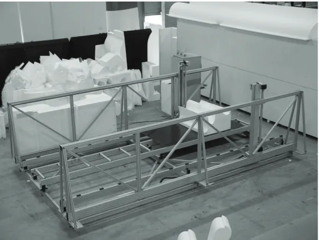
Advantages of HWC are, amongst others, its intrinsic simplicity and low energy use. Also, the speed for production of large shapes can be high compared to other material removing processes. It is in some cases considered a potential competitor in the field of three- to five-axis CNC milling, especially for products larger than the order of one meter and without much detail. Reasons are the lower cost due to reduced production time and reduced material usage. Disadvantages are some limitations in freedom of shape and level of detail. A photograph of a HWC machine is depicted in figure 1.2.
1.2
Introduction to rapid prototyping
‘Rapid prototyping’ (RP) is a terminology used to refer to techniques for creat-ing parts directly from ‘computer-aided design’ (CAD) models within a relatively short time. It is also referred to as ‘solid freeform fabrication’ (SFF). RP can be incremental or decremental [5]. Incremental RP uses material addition primar-ily and decremental RP starts with a raw block of material and shapes the final part by material removal such as milling. The incremental variant will be of main interest for this thesis. In the following, RP is used to denote the incremental form. The most well-known example of RP is stereo lithography, where parts are ‘printed out’ in three dimensions. In many cases, thin layers are created and subsequently or simultaneously fused together. The family of techniques using this principle is also called ‘layered manufacturing technologies’ (LMT). Materials used vary widely, but most often consist of (foamed) plastics or paper, although materials such as metals are used as well. The RP process is often characterized as an optimization between part accuracy and building time or cost. A significant production time reduction for prototypes as well as final products can be achieved, leading to an important role for RP in the design process [29].
Incremental RP processes can be generally subdivided in the steps shown in figure 1.3. In the following paragraphs, each step is explored. The second step is treated in more detail due to the relevance for the rest of this work as well as the fact that most systems make use of the same principles mentioned in that step.
Figure 1.3: Incremental RP process chain
The first step in the RP chain is to obtain a CAD model of the intended product. This can either be a solid or a surface model. The model can also be ap-proximated by a set of triangles that cover the surface, which is called ‘tessellation’ or ‘meshing’. An example is shown in figure 1.4.
Figure 1.4: (left) Exact CAD model of an aircraft body and (right) the tessellated version, using triangular facets
without presence of tessellation, which is then called ‘direct slicing’. When a tessellated approximation is used, the process is denoted as ‘tessellated slicing’. Whether or not direct slicing is used, the part is subdivided in a number of layers with finite thickness, bounded by two section planes. Use of a constant layer thickness is called ‘uniform slicing’. Varying the layer thickness as a function of local curvature, topology and other parameters leads to the term ‘adaptive slicing’, which can save the amount of layers considerably and hence cut cost as well. The ‘vertical’ or ‘build direction’, denoted by ~ez, is defined perpendicularly to the
section planes. The most basic techniques produce 2D-shaped layers, resulting in a so-called ‘staircase effect’ Take, for example, the two leftmost sliced shapes in figure 1.5. In literature, this has been defined as ‘zero-order slicing’. In general,
Figure 1.5: Overview of different slicing method combinations for an axisymmetric bell shape, depicted as one half of the cross-sectional shape for simplicity. Note that both efficiency and RP complexity increase from left to right.
Even more sophisticated is the use of ‘higher order’ slicing, yielding double curved layer side surfaces, but use of this technique is hardly encountered in literature and considered rare, as can be inferred from RP field overviews as in [29].
Figure 1.6: Schematic representation of a five-axis machine used for RP
RP technologies can also be classified by the layer thickness used. ‘Thin-layered’ is the de facto term used when referring to layers with a thickness (<= 1 mm) and thick-layered when a layer thickness of (>1 mm) is used.
The third step is transferring the sliced geometry to a machine and produce the layers from a specific process-related material. ‘Computer-aided manufacturing’ (CAM) is often tightly integrated with CAD in the RP process.
Fusing the layers is sometimes not necessary because the layers fuse during the layer creation process. However, some systems require bonding. This often requires additional automation and other means of help such as a guide pin and hole and connector systems, as shown in [1].
‘Thick layered object manufacturing’ (TLOM) is the term used to denote the fabrication of objects in the order of one cubic meter and larger, whereas traditional RP techniques are usually limited to a cross-section smaller than one square meter. HWC is suited for TLOM and also used for this purpose in practice. This work aims at combining HWC and TLOM as will be explained in the following sections.
1.3
Problem
ability to offer control of dimensional accuracy. Obviously, the surfaces generated with HWC deviate from double curved surfaces, requiring a good approximation method. Manual slicing often does not guarantee a part to be within the required tolerances. Most milling software inherently contain this kind of control by de-fault. Finally, it is important to realize that no matter how much automation is applied, the preprocessing stage still contains many aspects that require creative human thought which cannot be automated in a cost-effective sense due to the vast variety in nature of the customer projects involved. The issues mentioned above have lead to the project as described next, performed in cooperation with the University of Twente at the Department of Mechanical Engineering, Chair of Production Technology.
1.4
Scope of the overall programme
The foregoing lead to the start of the Protostyrene project which focuses at the issues mentioned in the previous section. This project encapsulates the Master project documented in this thesis. The top-level purpose of the project is to cre-ate an automcre-ated software tool that assists the pre-process engineer in defining an optimal slicing of a CAD model, saving time in the preprocessing phase consider-ably. Possibly, integration with CAM will be a long-term objective of the project as well. As preprocessing time generally constitutes the largest piece of the total product lead time and effort, this approach is considered justified. This objective is defined in a general way. The Master Project as described in the following section intends to take the first significant steps and sets a more specific objective.
1.5
Master Project objective
The Master Project objective is: To formulate and implement an automated method which subdivides an arbitrary two-manifold CAD model into parallel lay-ers in such a way that it maximally benefits from the four-axis hot-wire cutting process with a predefined accuracy, followed by the determination of the resulting accuracy with a physical demonstrator.
of rules and boundary conditions. The main focus involves finding a solution to the correspondence problem as well as finding a suitable error-approximation, combined with the creation of a physical demonstrator, which is used to get an indication of practical obtainable accuracy.
1.6
Thesis outline
Chapter 2
Background
In this chapter, the research groups and techniques currently employed are de-scribed, as far as applicable to the current project. The mathematical background of various subjects is treated in order to comprehend concepts and enjoy confidence in them.
2.1
Related projects
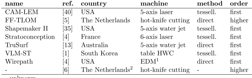
From literature, the advantages of first order adaptive slicing over zero order are well-known [14, 29]. For TLOM, only first- or higher order slicing are used and just a few groups have dedicated themselves to the development of systems capable of doing it. References or citations regarding more specific issues can be found throughout the rest of this work. The most well-known projects are presented in table 2.1. The projects stem from the past two decades, except the last one. Apart from these examples, a few other undocumented or otherwise non-publicly available projects may exist, as well as a range of non-automatized variants.
name ref. country machine method order CAM-LEM [40] USA 5-axis laser tessell. first FF-TLOM [5] The Netherlands hot-knife cutting direct higher Shapemaker II [35] USA 5-axis water jet tessell. first Stratoconception [4] France 6-axis laser tessell. first TruSurf [13] Australia 5-axis water jet direct first VLM-ST [1] South Korea table HWC tessell. first
Wirepath [4] USA EDM1 direct first
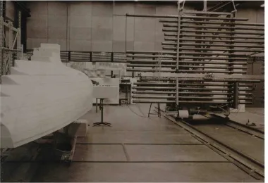
- [6] The Netherlands2 hot-knife cutting - higher - unknown
1 electrical discharge machining 2 see figure 2.1
Figure 2.1: Foam cutting machine at the University of Twente in the late seventies
2.2
CAD model import
Tessellated slicing has become very popular in RP. The file format used most often for import of a CAD model to a tessellated slicing system is the ‘stereo lithography’ (STL) file format. A STL file contains nothing more than a set of triangles without topological information related to the original CAD model. Various arguments in favor of and against STL exist. The most important are listed in table 2.2.
Advantages Disadvantages
de facto standard in RP topology loss simple algorithms for slicing required chordal error
basic and neutral file format limited functionality for complex parts large data set size
Table 2.2: Arguments in favor of and against STL
between the tessellation surface and the original CAD surface. Usually, the maxi-mum chordal error can be imposed by the user when tessellating the CAD model. Setting the chordal error one order smaller than the maximum allowed slicing error will eliminate significant contribution of tessellation errors, yet may increase the amount of triangles drastically. Due to the limitations of STL, alternative and more extended formats have been proposed [30, 38, 16], but have not yet lead to new widely accepted standards.
For research purposes, ‘finite element method’ (FEM) preprocessors can be used instead of STL. FEM tessellators are generally more robust, so the bulk of error checking is not necessary anymore. Besides, inter-triangular topology is preserved, the file size is reduced and import is faster.
On the other hand, ‘exact’ CAD file formats like ACIS, IGES and STEP provide a representation for solid and surface geometry as well using the ‘non-uniform rational B-spline’ (NURBS). When using the non-tessellated CAD geometry, this representation avoids the disadvantages of STL [13].
2.3
Decomposition, segmentation and build
di-rection
Before computational slicing can begin, decomposition and segmentation might be needed. Decomposition or ‘splitting up’ of a CAD model (assembly) into parts is usually very hard to automate [6]. The intended result depends on the purpose of the resulting physical model, which could, for example, imply that certain part of an assembly need not to be decomposed at all. The structural strength of the individual components is also an aspect when decomposing, just like accuracy, economical aspects and specific process-related constraints.
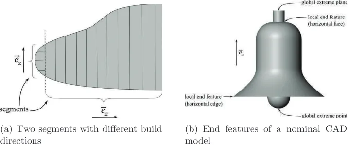
(a) Two segments with different build directions
(b) End features of a nominal CAD model
Figure 2.2: Segmentation and end features
detection, as in figure 2.2(b), can assist the segmentation process [33, 26, 23, 19, 4]. These subjects will not be discussed in further detail. Here, the build direction is assumed constant for each single segment. This could, of course, be generalized to a varying build direction throughout a segment, giving more freedom, but this would increase the slicing process complexity both theoretically and practically.
2.4
Slicing
Although every type of (non)parametric surface has its own mathematical descrip-tion, most CAD package geometry kernels are able to offer common interfaces for arbitrary surface types, along with integrated intersection algorithms, greatly fa-cilitating the slicing procedures. The need to program, for example, intersection functions for each type of surface is therefore not necessary.
Computational slicing exists in many varieties. In the current project, only adaptive first-order thick-layered slicing is considered due to the corresponding properties of the HWC process. The slicing step is of particular interest and therefore treated in more detail. The most important part of slicing is the problem of surface reconstruction by ruled surfaces from a set of intersection contours and optionally the original surface. The next section treats this problem, followed by sections describing tool path generation, layer thickness estimation and actual error estimation.
2.5
Correspondence problem
This section will presents a mathematical description of the correspondence prob-lem. Next, implementations of solving the correspondence problem are given.
2.5.1
Ruled surfaces and correspondence
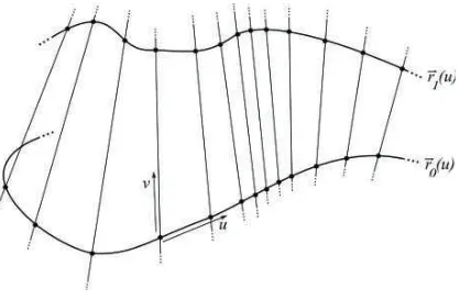
As mentioned before, ruled surfaces play a role in both HWC and RP. Mathemat-ically [9], a ruled surface R can be expressed by straight lines, ‘rulings’ or ‘genera-tors’ joining corresponding points on two space curves~r=~r0(u) and~r=~r1(u) in R3
, also known as directrices. The expression can be given in the following form:
~r=~r(u, v) = (1−v)r~0(u) +v ~r1(u) (2.1) A ruled surface is depicted in figure 2.3. When the rulings are initially unknown, it is convenient to express the contours as regular parametric curves:
Cb(ub) andCt(ut),
Where subscriptb stands for base andtfor top, as used throughout the rest of this work. Next, allow ub and ut to be changed by Ub : x 7→ub and Ut :x 7→ ut with
the constraint that U0
b(x) > 0 and Ut0(x) > 0, yielding regular parameterizations.
The ‘regular’ property of the parameterization ensures that no unnatural self-intersections occur. Now,Ct can be reparameterized by ut(ub) = Ut(Ub−1(ub)) and
hence the contours can be expressed as
Figure 2.3: Ruled surface
The rulings have now become a result of this functional relationshiput(ub). Using
the arc length as parameter, finding an acceptable or optimal solution for this relationship simply involves solving the ‘correspondence problem’. Stated other-wise, it deals with the topological adjacency relationships between the contours. That is, determining which point on the upper section contour corresponds to an-other point at the lower contour. Next, assume each curve to lie on a plane and assume that these planes are parallel. Then, the mechanical equivalents of these mathematical concepts can be identified as in table 2.3.
Mathematical Mechanical
top directrix = top contour
base directrix = base contour
ruling = (approximate) wire location at specific time
functional relationship = correspondence or (approximate) tool path
Table 2.3: Mechanical equivalents or mathematical concepts
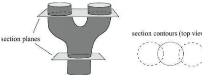
Solving the correspondence problem is severely under constrained and therefore challenging. Stated more loosely, an infinite number of (ruled) surfaces can form the surface connecting the contours. As an example, different correspondence solu-tions for two circular intersection curves are shown in 2.4. The problem also exists in many other fields such as CT-scan imaging. In those fields, only the contours are available. Most literature focuses at reconstructing a tessellated surface from a set of contours only. However, for RP, the original surface is available as well by a (tessellated) CAD model, giving additional information for correspondence solving.
Figure 2.4: Two correspondence solutions yielding a cylinder (left) and a hyper-boloid (right)
Figure 2.5: A simple example of branching
2.5.2
Implementations
The following implementations make no use of the original surface and base their solutions on the presence of contours only. Subsequently, two implementations that do use the original surface and topology are presented.
In one of the earliest publications, Keppel [18] defined the correspondence problem as a graph theory problem (figure 2.6). The optimal path in a graph was defined by using a cost function maximizing the resulting volume of the contained polyhedron. Later on, similar methods were used minimizing surface area [10] or summed span length. A span is defined as a line segment which represents a correspondence between two points onCb andCt. All methods are rather arbitrary
due to the under constrained nature of the problem. The minimum surface area is used often, although is has been proved that this generally leads to hyperboloid shaped solutions and thus, in general, not properly representing the original surface [3]. Most of these methods are of order n3 or sometimesn2log(n), wheren is the
number of sample points at one of the contours, assuming an approximate equal number of points on both Cb and Ct. Note that this approach and others using
triangular facets result in a so-called one-to-many correspondence. That is, one point on Ct can correspond with multiple points onCb and vice verse.
Figure 2.6: Graph theory approach to correspondence solving. The graph path at the right represents a possible solution as depicted left.
Figure 2.7: Advancing front meshing technique used for surface reconstruction.
Cohen et al. [7] proposes an order n3 contour matching scheme based on the
differential properties of the curves. The technique tends to be feature preserv-ing, twist- and self-intersection free. It matches the directions of the unit tangent vectors. The optimal solution is one with maximum summed dot products (pro-jections) of each pair of corresponding tangent vectors, see also figure 2.8. This method yields good results when using contours that do not differ too much from each other. However, in many cases it proposes a solution that does not represent the original surface with sufficient accuracy.
Figure 2.8: Tangent matching result
In the CAM-LEM project, Zheng [40] solves the correspondence problem by creating a one-to-one relationship between points at two consecutive sections, usu-ally at high resolution with ‘almost’ ordern complexity. The principle is depicted in figure 2.9. Half way between two sections, an additional middle section is used
Figure 2.9: Example of the spring system used by Zheng to find a minimum energy solution.
to generate a set of sample points. At each of those points, a guided spring rod, connected with a ball-joint as shown. The rods represent the correspondence spans here. The springs are linear springs with no torsion stiffness. Both rod ends are connected toCb and Ct with a sliding ring connection. The strain energy function
of a single span is given by:
Ei(sb,i, st,i) =
where the distance D~ is defined as
~
Di(sb,i, st,i) =m~i−~ai(sb,i, st,i) (2.4)
with~ai as the acting point on the span andm~i as its attractor point on the middle
section. ~ai can be chosen to be either the middle of the span or the closest point
to its attractor. Distance L~i can be expressed as
~
Li =~eb,i−~et,i (2.5)
The summed energy function then serves as the objective penalty function. The algorithm used makes sure the spans never cross each other, making the system non-linear and requiring creative solutions. Using a wavefront method, the system uses relaxation of the objective function. However, spans may touch each other somewhere on Cb and Ct, yielding a one-to-many correspondence relationship
be-tween Cb and Ct. When this is not desired, digital filtering techniques can be
figure 2.9, which is ‘trapped’ behind a sharp corner at the top section. Solutions for this issue are mentioned by Zheng as well. The ratio of stiffnesses chosen should be such that the system converges fast enough yet stays stable. The ratio is also a compromise between approximation accuracy and ruled surface smoothness. The initial positions of the critical spans as used by Zheng were determined partially by existing techniques as well as following common logic. As good choice also speeds up the convergence of his solution. Zheng also offers various extensions and vari-ations to the method proposed, each with its specific problems and opportunities.
The last correspondence solving method addressed is called ‘topology traver-sal’. It uses the nominal CAD geometry topology to create spans at such locations that most features, such as sharp edges, are preserved [34]. It is depicted in figure 2.10. Simply stated, the algorithm determines which intersection contour segments at the ith section matches a segment at section i+ 1. When topology gets more
complex, this method fails easily and needs user interaction or other methods such as those mentioned earlier to find a solution.
Figure 2.10: Usage of original CAD model topology for correspondence generation
After defining the spans using either of the previous methods, a set of two consecutive spans now bounds a ruled surface patch which is parameterized to define the correspondence between the spans. Each patch is linearly interpolated in terms of arc lengths. Applying it as in figure 2.11 by expressing the top parameter as a function of the base parameter, we get:
st(sb) =st,i +
st,i+1−st,i
sb,i+1−sb,i
(sb−sb,i), (2.6)
with sb,i ≤sb ≤sb,i+1.
Figure 2.11: Base and top curve with spans indicating the correspondence solution at sample locations
2.6
Tool path generation
Every correspondence solving method mentioned before can be used to generate a one-to-one correspondence between Cb and Ct. This is often highly desirable
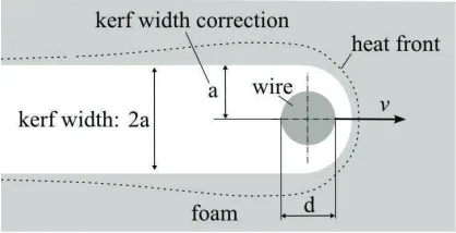
for tool path generation as excessive burning is avoided this way. When a one-to-one correspondence exists, this can be used directly to generate the tool path. However, in order to obtain high accuracy, compensation for kerf width (figure 2.12) should be taken into account by the kerf width correction (KWC), which lies in the order of 1 mm for HWC. Further treatment of optimal KWC calculation goes beyond the scope of this work.
Figure 2.12: Kerf width geometry
Assuming one-to-one correspondence, the result after assembling the layers is depicted in figure 2.14 on the far left. However, when triangulation was used for correspondence solving, the correspondence has a one-to-many relationship and the denominator in equation 2.6 evaluates to zero in many cases. Direct use of this correspondence can result in excessive burning of the material due to low local wire speeds. In this case, another approach is desirable, as used by the VLM-ST group [24]. Given a layer with one-to-many correspondence, the set of facets as obtained from correspondence solving (not a STL mesh!) is intersected half way
Cb and Ct, resulting in Cm. The tool path orientations are then calculated as
~ni×~ti, as shown in figure 2.13. This method can also be applied to the exact CAD
surface without solving for correspondence as a separate step. In that case, think of the facets as in figure 2.13 to be replaced by the original CAD surface.
Figure 2.13: Toolpath generation using a one-to-many correspondence
section contour height does not coincide with the original contour itself. Another kind of defect, this time for a single layer (figure 2.15) results in an undercut at the corner of a faceted part. The Truesurf [13] project offers both the arclength parameterization usingCb and Ct and the cross-product method using Cm.
Tightly connected to the cross-product method in literature [13] is the offset, required to meet zero in- or outside tolerances, depending on the post-processing available. Figure 2.14 briefly shows different possibilities. The methods for this subject are beyond the scope of this work.
Figure 2.14: Results after generating tool paths and fusing layers together
When the maximum tool angle is exceeded, various solutions can be offered. Brink et al. [4] approximate a ruled surfaces which is too steep by one having the maximum tool angle. This would require additional post-processing. Stated differently for the case of HWC, the layer geometry is adjusted to conform the maximum wire angle.
2.7
Layer thickness estimation
The ruled surface approximation of an arbitrary nominal parametric surface S
Figure 2.15: Triangular tessellation with corner defect, caused by generated tool path
maximum distance between S and the approximating ruled surface R. Although
δ is often not defined accurately, it is usually measured along the normal~nS of S,
which is also done here. Variations exist [28] where the user can define multiple values for δ for different model regions, but this is omitted here. Here, δ repre-sents the maximum allowed ‘normal deviation’, which may also be known as the ‘chordal error’. With the use of adaptive slicing, layer thickness is often deter-mined using the curvature of S in build direction together withδ. In regions with high curvature, this generally results in smaller layer thicknesses than in regions with low curvature. In literature, a description analogous to the following can be found in [15]. The procedure is described in the following paragraphs, introducing the parameters as summarized in figure 2.16 top-down.
Figure 2.16: Parameter dependencies
Suppose that at a given moment in the slicing procedure, the next layer thick-ness needs to be established. The top section of last finished layer now serves as the base section for the next layer. Figure 2.17 shows a single sample pointXi on
the new layer base contourCb with known~nS,i. Build direction~ez is known as well
purpose, a ’normal plane’Pi is defined, spanned by~nS and a unit ‘direction vector’
~
di, so the normal of Pi at Xi can be expressed by
~nP,i =~nS,i×d~i (2.7)
In literature [15, 21], substitution d~i =~ez is often used, defining P as the ‘normal
vertical plane’ (NVP). The following applies to the more general case where d~i is
Figure 2.17: Curvature determination in plane P, here spanned by~nS and~ez
not necessarily coincident with~ez. Although this generalization was not explicitly
found in literature, it is still mentioned here because it is strongly related to existing thickness estimations using substitution d~i = ~ez. It involves geometry
in Pi, as shown at the right of figure 2.17. Denote the curve that results from
the intersection of S by Pi as CS,i, the actual intersection of R by Pi as CR,act,i.
Now approximate CS,i at Xi by a circle with radius ρi whose value is determined
shortly, and approximate CR,act,i by the linear ‘estimation’ CR,est,i. Using these
approximations, geometric considerations in appendix A then help to show that the ith
sample based layer thickness estimation ti can be expressed by
ti =
to be determined in order to evaluate expression 2.8. In general, the radius of curvature of a space curve is the reciprocal of its curvature:
ρ= 1
The curvature of CS,i at Xi is defined as the ‘normal curvature’ κn,i. Its value
depends on the direction of ~ti along CS,i, which is determined by the rotational
orientation of P about ~nS,i. This orientation is defined by d~i. Theory for
deter-mination of κn for parametric surfaces is given in appendix B. The result can be
represented by
with E, F, G and L, M, N representing the first and second fundamental matrix elements of the parametric surface, respectively, which are constants when evalu-ating curvature in an arbitrary direction at a specific point Xi. Using ~r(u, v) to
describe S,du and dv can be solved from
~ti =
where the subscripts denote evaluation at point Xi. Note that the actual
inter-section curve does NOT have to be calculated for the steps above. Vector~ti can
easily be obtained after projection of the direction vector on the tangent plane (not shown) along S atXi:
In the relations above, the estimated section curve of R is assumed to be a straight line as in figure 2.17. However, this will generally not be the case. Remember that this procedure is used only for layer thickness estimation. The correspondence solution is most probably determined after thickness estimation, possibly resulting in a different -nonlinear- intersection curve. Take, for example, a hyperboloid as shown at the right of figure 2.4. Assume the correspondence solution to be represented by the same figure. use the hyperboloid as the nominal shape with substitution d~i =~ez along the axis of symmetry. Now CR,act deviates
from CR,est in the NVP. This implies that the actual error e, measured along~nS,
might exceed δ. Apart from the deviating tool path, the difference in actual error might also be a consequence of the circular approximation. Both contributions are visible in figure 2.17.
The procedure can be repeated for a set of sample points on Cb. Each sample
yields a layer thickness estimation, based on the local geometry. The new layer thickness estimation can now be conservatively chosen from n samples as
t∗ = min{t
i | i= 1. . . n}, (2.14)
Where t∗ denotes the critical thickness. The amount of samples and their
The maximum and minimum normal curvaturesκn,1 andκn,2at a surface point
are called the principal curvatures. It can be shown [9] that the principal directions, corresponding to these curvatures, are orthogonal. Now define the orthonormal ‘principal frame’ (~e1, ~e2, ~nS) with ~e1 and ~e2 the normalized principal directions.
When the principal curvatures and -directions are known, the normal curvature in an arbitrary direction can be obtained by application of the Euler formula:
κn(φ) =κn,1cos2(φ) +κn,2sin2(φ) (2.15)
where φ is the angle in the tangent plane from ~e1 to ~t in the principal frame.
An example is depicted in figure 2.18. In this case, κn,1 = R1 and κn,2 = 0. This
relation has not been encountered by the author in RP literature, although it makes use of the principal curvatures which play a key role in the field of differential surface geometry. In spite of its simple appearance, derivation of this relation requires a lot of effort and goes beyond the scope of this work, but was done by Euler in 1760. In general, the principal curvatures can be evaluated easily once the fundamental matrices are known. Once the principal curvatures are known, checking for singularities is not necessary anymore, in contrast to equation 2.11.
Figure 2.18: Principal curvatures
Banerjee et al. [2] substituted~i not only by~ez, but also by~e1 and~e2, assuming
the tool path to lie in one of these three directions during the entire cut. However, range limitations of the cutting machine would often render such an approach less suitable. It was concluded [2] that taking the ‘maximum absolute curvature direction’ (the direction corresponding to the principal curvature κn,pr for which |κn,pr| = max{|κn,1|,|κn,2|} holds) yields a maximum number of slices but the
smallest volume difference error. The volume difference error is described in section 2.8. The ’minimum absolute curvature direction’ yields a minimum number of slices but the largest volume difference error. The NVP-approach comes out as a compromise of the two.
2.8
Error analysis
Hope et al. [15] identify a representation for the actual error other thanδ. The maximum distance in the layer plane, , is taken as a measure for the volume dif-ference between the nominal and approximated model, while theδusually presents a better roughness representation. Figure 2.19 illustrates bothδ and . When the nominal surface normal approaches the build direction, is less representative for volume difference. In that case, cusp height gives a better representation for both surface roughness and volume difference.
Figure 2.19: Two measures of error: cusp height δ and layer plane error.
Koc [20] proposes a marching algorithm which samples the actual error. The sampling is taken along an intersection curve, created by intersection of a plane and the nominal surface. The plane is spanned by the vector between two corre-sponding points P and P0 and the average of~n
P and~nP0 as shown in figure 2.20.
The curve itself is not calculated, but the sample points are obtained through the
Figure 2.20: Marching algorithm
differential properties of the surface. The samples are taken from the base section to the top section. Sampling size and distribution do not receive much attention. Kumar and Choudhury [22] proposes a different approach. The ruled surface is approximated by a set of parametric bilinear patches, also known as cubic spline patches. For each bilinear patch, the corresponding model surface patch is iden-tified and sampled in u and v direction. Next, the error along the nominal model surface normal ~nS at the sample points is evaluated by line/patch intersection.
Figure 2.21: Bilinear patch approximation
risk of intersection with a patch point outside the patch area is present, possibly yielding misleading results. This effect should be taken into account. An alterna-tive approach mentioned is to determine the error along the normal of the bilinear patch (not shown in the figure). It was observed that application of this approach yielded more and thus thinner slices than the situation with only the layer thick-ness estimation used for error estimation. This is as expected as layer thickthick-ness estimation has its limitations as discussed in section 2.7.
The difference in volume between exact CAD model and the sliced approxi-mation also poses an error quantifier. This can be evaluated per layer or for the entire model. Geometric modelers usually offer tools in order to calculate this. However, this approach only gives global information. The difference in volume may be very small, indicating valid solution, yet locally, the actual error may exceed user-defined limits.
The angle between the ruled surfaces of two subsequent layers may also serve as a measure of error. When a smooth body is required with little post-processing, this measure of error may be appropriate.
The methods above are mostly based on sampling and thus represent an esti-mation of the true maximum error. Higher accuracy comes with increased compu-tational cost. In order to come up with a suitable error estimation, the objective must be known first.
2.9
Physical fabrication
it to the machine, then cut, etcetera. Most of the time, machines do not facilitate this. It would lead to high operator cost when repeated often and cause tedious labor. Some systems are supplied with a sheet feeder, which automatically feeds the cutter with an uncut sheet of paper, foam of whatever material is used. When using adaptive slicing, this requires ordering of the sheets as sheets with different thicknesses follow each other.
The VLM-St project [1] mentions the use of guidance pin holes in the part for accurate alignment of the individual layers. Also, connectors can be generated by software where multiple disconnected contours are cut in one layer, just for proper positioning as well.
The fusing of the layers can be done manually or automatically, but literature does not mention much about this subject regarding TLOM systems.
Chapter 3
Analysis
This chapter contains the requirements for the design of a RP tool for the HWC process, based on the demands of 3EL-Company and additional limitations. Next, decisions are made regarding the best suitable methods to meet these requirements. First, cases are presented to give an impression of typical shapes used as input for slicing.
3.1
Typical cases
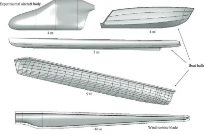
A few examples of various shapes from the 3EL-Company archives are shown in figure 3.1. An example of a wind turbine blade model is depicted at the bottom of the figure. Most of the examples are boat hulls, but the upper left example is the bare shape of an experimental aircraft body, which will serve as a demonstrator throughout this thesis.
3.2
General requirements
A set of requirements for the overall programme was set up and is presented here. In order to get an effective slicing tool, it must satisfy the following global require-ments:
• generate a 2.5D ruled surface approximation of the exact CAD model,
• perform layer thickness optimization,
• comply with a user-specified tolerance field,
• preserve features such as sharp edges as much as possible,
• offer generation of a continuous part surface (no saw-tooth effect),
• offer user-defined uniform slicing,
• include feasibility checking of the wire angle,
• include surface quality check.
advan-Figure 3.1: Various examples which have been fabricated with HWC. Note that the examples are drawn in different scales.
tageous for the HWC engineer to be able to, for example, simulate various slicing scenarios with variable tolerance values and evaluate the corresponding cost. How-ever, the cost aspect is not analyzed here. Furthermore, the software tool can assist in decisions regarding manufacture feasibility.
3.3
Master project requirements
Decisions have been made regarding in- and excluded requirements for the Master project, based on fitness for automation and available development time.
Included requirements:
• offer first order surface approximation,
• offer adaptive slicing,
• offer user control over available layer thickness set,
• offer a user-defined build direction,
• preserve topology (sharp edges in correspondence solving),
• generate continuous part surface (no saw-tooth or staircase effect),
• offer actual error evaluation: normal deviation,
• offer a check of the maximum machine wire angle,
Most important non-included requirements:
• CAD model decomposition and segmentation (e.g. from end features),
• automatic calculation of optimal build direction,
• varying build direction through the model,
• zero order slicing,
• feasibility checking w.r.t. part size and -location in machine,
• branching in build direction,
• correspondence solving with user interaction,
• zero in- or outside tolerance fields,
• generation of pilot pin-and-hole and connectors,
• specialized CAM file format (with correspondence info),
• graphical user interface.
Both decomposition and segmentation have been excluded from the master project for the reasons mentioned in section 2.3: high expected development cost and lim-ited value for the proof of principle.
The determination of the optimal build direction is assumed to be a relatively simple task for the user, which is plausible with respect to shapes such as shown in figure 3.1. It has therefore no primary priority.
The build direction is kept the same through the segment because of increasing complexity of technical issues, both practical and computational.
Zero order slicing is left out as it does not make good use of the four-axis HWC process, although it could be implemented with relative ease once computational first-order slicing is possible.
Part size and location in the machine also affect feasibility and are left to the user’s responsibility as well. It would, amongst others, require the software to have knowledge of the overall machine dimensions and kinematics, which could be variable when the tool is used for production on different machines, demanding a proper machine database. Also, the location in the machine can be optimized for, just as optimally nesting the layers in a source sheet.
Branching is left out as it can be avoided easily by manual segmentation. It would also require specific attention as mentioned in section 2.4: Many of the ‘most intelligent’ algorithms fail miserably in even the more simple cases. Apart from this, no primary demand is present as can be derived from figure 3.1.
Correspondence solving with user interaction would also require further anal-ysis, yet this is expected to be manageable. However, the possibly complex user/automation interaction would be of primary interest here, which does not contribute to general insight into the slicing process in this Master Project.
Zero in- or outside tolerance are excluded as it requires specific attention. It requires methods like offsetting section contours. However, the solution used also depends on the requirement whether or not a continuous outer surface is required or not, as explained in section 2.6. A possible workaround can be offsetting the original CAD model outer surface with the maximum allowed cusp height. Next, the offset model can be sliced using the same cusp height as a measure of maximum allowable normal deviation.
assumed to be alignable by themselves. When one or more sharp edges are present, this is generally the case, although it must be treated with great caution. Usually, alignment shapes can be integrated with the part design.
Finally, a specialized CAM file format design is left out. This file should con-tain enough information to provide the machine controlling soft- and hardware with cutting data and therefore requires cooperation of the HWC machine manu-facturer.
3.4
Practical requirements and constraints
The machine used for the project is a Step Four PC-CUT 5000 series HWC ma-chine, made in Austria. It is shown in figure 1.2.
PC-CUT 5000 machine properties:
• four independently controlled axes,
• manual variable distance between the portals (250-5000 mm),
•max. dimensions in the layer plane: 5400 x 1460 mm (equals raw block sizes),
• max. wire angle: set at 45◦ (in software).
Machine software properties:
• dedicated control,
• very basic 2D CAD environment,
• simulation (along 2D contours),
• DXF (2D contours) / HPGL (very basic) import,
• Step Four SCF-file format with correspondence information,
• operating system: DOS.
The 2D drawings can best be imported through the DXF interface, but remain without any information regarding correspondence relationships or KWC. Corre-spondence is subsequently applied either manually or automatically by contour matching using a minimum change in contour angle between two successive poly-line segments. This easily leads to solutions that are not intended by the user or even unacceptable surfaces. It would require extra manual effort for the more sub-tle regions of correspondence. Tool path calculation is done using linear arc-length parameterization as described in section 2.6.
In order to review the computational slicing process, the user must obtain a file with the results. This requires that the slicing process documents its progress in a log file, allowing the user to change input parameters based on the log file data.
To summarize, the following additional requirements are defined:
• offer DXF file export option,
• offer log file generation.
It was decided to let the user set a maximum allowed wire angleθmax which is the
maximum angle between the wire and the normal of the portal planes as shown in figure 1.1. The actual wire angle θ must not exceed this value. The largest actual wire angle is denoted by θ∗. When no layer thickness solution is found for
θ∗ < θ
max, the part is defined as not feasible. Other solutions can be proposed
in-stead, e.g. involving cutting with lower wire angle than actually needed, resulting in additional post-processing. These solutions have been omitted here.
3.5
Methods
In this section, the chosen solutions for the various steps in the RP chain are presented and substantiated.
3.5.1
CAD model import
The choice between direct and tessellated slicing caused quite some discussion with various arguments put forward. The essential characteristics of both are captured in section 2.2. It was finally decided that the direct slicing method is favorable. The most important reasons are:
• chosen method for correspondence solving (see below),
• strongly reduced development/implementation time.
3.5.2
Correspondence problem
In general, user interaction remains inevitable for obtaining the correct solution of the correspondence problem when confronted with geometries are more complex. Assuming not only contour data but also the original surface to be present, this statement still holds, although more information is available. The problem remains ill-constrained.
3.5.3
Tool path generation
Once the correspondence has been determined, the tool path is generated assuming a one-to-one correspondence. For layer L, define a base- and top section contour
Cb and Ct, both parameterized by arc lengths sb and st, respectively. Assume a
known mapping from sb to st, defined by the correspondence solution:
F :sb 7→st. (3.1)
A contour generally consists of multiple contour segments. A segment is described by a parametric curve, bounded by a start and end parameter. Let F take this into account when evaluating. At the ith location ofs
b, the coordinates on
base-and top contour are, respectively,
~rb,i =Cb(sb,i) (3.2)
and
~rt,i =Ct(F(sb,i)), (3.3)
Define~c as the unit ruling vector (see section 2.5.1 for the definition). At sb,i, we
get
~ci =
~rt,i−~rb,i
|~rt,i−~rb,i|
. (3.4)
Using this approach in a discrete or continuous sense, the tool location and orien-tation can be evaluated along the entire boundary ofL. That is, without any kerf width correction applied.
3.5.4
Error analysis
Sampling of the normal deviation of the nominal surfaceSis chosen to represent an estimation for the actual error e. The maximum absolute actual error is denoted bye∗. The normal deviation or the distance along normal~n
S,i to the ruled surface
intersection point is calculated at a user-defined sampling rate (see figure 3.2). Define Rset as the set of rules surfaces approximating S at layer L. When the
thickness of L and correspondence solution have been established, an intersection half way the section planes of Cb and Ct is created, yielding a contour Cm on S
which is then sampled by arc length s. The choice of the section to be half way the layer is chosen because that is the location where e is assumed largest, given the fact that the normal error equals zero at Cb and Ct. At each sample point Pi,
used to intersect the surfaces in Rset of L. The distance along l between Pi and
the geometric intersection~xi of Rset then represents the local actual error ei. Note
that the line can intersectRset multiple times so the correct intersection should be
selected.
Figure 3.2: Normal deviation sampling along nominal surface normal
The error check can be stopped once ei > δ. The procedure can be repeated
for multiple section heights.
3.5.5
Surface quality
Using HWC, manufactured part surface regions with relatively low local wire speed can be characterized by a higher surface roughness, higher surface foam density or excessive burning, depending on orientation with respect to gravity, causing buoyancy of hot air to form ‘chimneys’ in the foam in extreme cases. The cause of this phenomenon is schematically illustrated in figure 3.3. The amount of melting
Figure 3.3: Schematic correspondence solution including regions of low wire speed
can be characterized by the arc length ratio . The arc length ratio is defined by
i ≡
min{|∆st,i|,|∆sb,i|}
max{|∆st,i|,|∆sb,i|}
(3.5)
and the minimum arc length ratio at a single layer is defined by
∗ ≡min
Surface roughness typically significantly increases when is in the range of 0.6 - 0.2. At lower values, which approach the case of one-to-many correspondence, excessive melting can occur at the contour with the smaller arc length.
A part of the solution is to compensate for the kerf width. However, KWC cannot always fully compensate for excessive melting behavior. An accurate way of KWC calculation is important, but left out here.
Another solution to excessive burning is, as mentioned in section 2.5, applying digital filtering techniques to reduce low wire speeds. However, this will probably result in a surface that is further away from the optimum, possibly canceling out some of the optional previous correspondence optimization effort. This solution is particularly useful when the ratio approaches zero or infinity, values where the wire will progressively burn into the foam surface.
It was decided to let the user define a minimum allowable arc length ratio
min, based on his experience. When this constraint cannot be met, the part is
defined as not feasible. In other words, this constraint tries to force the solution into one that avoids a one-to-many correspondence.
3.5.6
Layer thickness estimation
In order to arrive at an optimum layer thickness as fast as possible, an accurate thickness estimation is needed. The layer thickness estimation is made with the method from section 2.7. Using an iterative process, the optimal layer thickness is determined.
It was decided to limit the thickness solution space to a user-defined set of available sheet thicknesses. This yields the following advantages and limitations.
Advantages:
• the user can choose and limit the thicknesses for practical constraints
• the algorithm can be kept simple
Limitations:
• a custom thickness (to take end features into account) is not available
• human factor in choosing thickness set
• sub-optimal resulting layer thicknesses
In practice, using the current machine setup, use of too many different thick-nesses is error-prone. Until present, most products have been manufactured using just one or two different thicknesses. It could be the case that after the computa-tional slicing process, the user is not satisfied with calculated layer thicknesses for various reasons. In this case, the set can be modified using the new insights and the slicing process can be run again.
Denote a ‘sheet thickness database’ containing the available user-defined thick-nesses by
Let a sample be denoted by subscript s. In principle, a layer thickness esti-mation, denoted as ts, can be evaluated atn samples on base contourCb for each
iteration, according to the curvature relations from section 2.7. A proper sample set might be generated automatically. Here, the samples are be homogeneously distributed at a user-defined rate. Define the sample set as
X ={s1, s2, . . . , sn|si ≥0∧n≥1∧sn <sup(sb)}. (3.8)
An iteration is denoted by subscripti. Using the foregoing relations and data, the
ith iteration for layerL can described. In order to do this, the direction vector d~
s
(section 2.7) must be known. Now use substitution
~
Note that at i = 1, correspondence F (equation 3.1) and hence ruling vector
~c(sb) are unknown. Hence,~c(sb) is approximated by~ez. In the next iterations, F
is known so ~cs can be evaluated using equation 3.4. After ts-evaluation at each
sample, t∗ is obtained from equation 2.14 as t∗ = min{t
s |s = 1. . . n}. For this
iteration, a curvature-based TDB-index is then conservatively obtained by
˜
with tL as the layer thickness of L. The choice for a unit change is based on the
assumption that T(Ii−1) lies near the optimum layer thickness, although this is not necessarily the case. It is also assumed that
which are both assumed to hold at least in the limit tL ↓0. To be determined is
∂θ∗
∂tL
, (3.14)
which is derived from the sign of the κn and normal vector orientation at the
sample point at Cb containing θ∗.
Finally, the TDB-index for iteration i of L is determined:
Ii =
After thickness determination, a new section is created at an offset from the base section by the new thickness. This section can then checked for a single closed contour. Next, the correspondence forLcan be solved. Finally, ∗
i,e∗i andθi∗ can
be evaluated and stored together with the iteration i.
Notes:
In some other RP implementations, the layer thickness is unchanged when
e∗
i ≤ δ. Although the layer is acceptable, it may not be optimal. It is possible
that t∗
i an hence also T( ˜Ii) are too small, based on the limitations of κn-based
thickness estimation. However, here, thickness is increased. This may eventually save cutting time because thicker sheets may be used.
When θ∗ > θ
max, the thickness must be changed in direction of decreasing
wire angle. Usually, this means that a thinner layer is desired. However, this is not necessarily the case, as near the nose of the upper leftmost case in figure 3.1. Building from left to right using the same case, the surface at the nose becomes less steep with respect to build direction. In that case, a larger layer thickness reduces θ yet may increase e∗. When, in this case, already e∗ > δ, ˆI
i becomes
indeterminate and the iteration deadlocks, rendering the geometry not feasible for production. A better manual start plane location, further away from the nose tip can solve this problem.
The next example is given to illustrate the merit of multipleκn-based thickness
estimations in the consecutive iterations. Take a small patch which resembles a piece of a cylinder (see figure 3.4) from nominal surface S. At sample point P, one would intuitively predict a thickness of infinity, based on the given shape, build direction and expected tool path, denoted by the plotted spans. However, iteration 1 determines the κn-direction using substitution d~1 = ~ez. This yields
κn,z > 0, locally yielding a finite (too small) thickness estimation. Next, the
correspondence is solved for, parameter evaluations are performed and iteration 1 is finished.
Iteration 2 might offer a better estimation. Using the solved correspondence from iteration 1, depicted by the spans, substitution d~2 =~cP is applied, yielding
κn,c = 0 and infinite estimated layer thickness. Note that topology should then
dictate a maximum to the thickness.
Figure 3.4: Approximation of surface (not shown) around P by a cylinder. The subscripts denote the first two iteration numbers
‘skew cylinder effect’. Remember that t∗ is ultimately used for layer creation. This means that the local over- or under-estimation of layer thickness does not necessarily lead to a bad thickness estimation.
It was decided to omit further use of improved κn-based thickness estimations
for the third iteration onward. Instead, only unit increment DB thickness changes are used. This decision is based on the assumption that the directional change of
~
d from iteration to iteration is relatively small after iteration 2. In other words,
~c is assumed not to change significantly. In general, this might not be the case. However, this was not investigated. It strongly depends on the shape and topology of the input model. Also, it should be remembered that a κn-based thickness
Chapter 4
Implementation
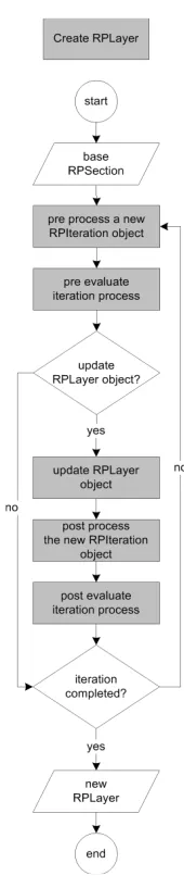
This chapter describes how the chosen methods are implemented in a custom-built program attached to an existing CAD software package. The program is called ‘Solidfoam’. The program structure is presented in a Class diagram. Next, the program execution flow is described using charts. A more exhaustive set of flow charts is presented in appendices C and D.
4.1
Programming approach
It was decided to use an existing Windows based CAD package to implement the RP tool. CAD software developers have been realizing for a long time that customers need customization to the package and therefore offer an API (Appli-cation Programming Interface) to tailor and extend the software as needed. Solid Edge (SE) from UGS and Solidworks (SW) from 3DS , two affordable mid-range CAD packages, were candidates. Solid Edge is used by 3EL-Company and Solidworks by the University of Twente. Both use the same Parasolid geometry modeling kernel. Although Solid Edge was preferred as it is the primary CAD package at 3EL-Company, Solidworks was eventually chosen for implementation, using the arguments in table 4.1.
feature or facility SW SE no. of spans (using API) >20 3 (max) 3D drawing possible yes no record macro’s yes no API user basis small big
Table 4.1: Differences between Solidworks and Solid Edge which affect implemen-tation
speed and sometimes difficult interoperability with legacy COM components. The chosen system architecture is depicted in figure 4.1. It is a rather conventional architecture. The proxy is implemented as a class, working as an interface for all external API-calls. It also wraps API functions by more intuitive or more suitable defined functions. Note that the geometric kernel cannot be approached directly but through a restrictive API. Alternative architectures with different operating system or CAD-system architectures could be more suitable for research purposes, but this discussion is omitted here due to the practical context in which the project was set up.
Figure 4.1: Conventional software architecture
Note that here, no graphical user interface was developed. Parameters can be changed in the source code only, which, together with several other restrictions, leaves the application in a prototype phase. All operations are performed in the Solidworks part environment using a single part.
4.2
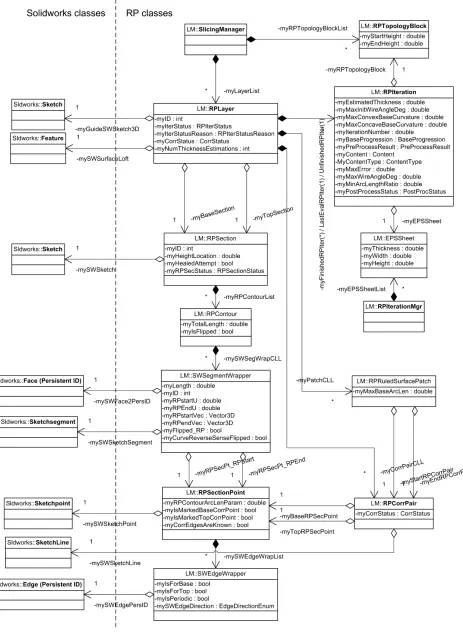
Application Class diagram
The program data structure can be represented by a class diagram. It represents reality in a relatively intuitive manner, as many classes can be compared to what they represent physically, geometrically or mathematically. Figure 4.2 shows the simplified diagram containing the most important classes, ignoring functions and less relevant attributes. The left column of classes represent Solidworks classes that are referenced by Solidfoam. The diagram is commented in a top-down manner. Starting with the ‘SlicingManager’ class which controls the slicing process, it is shown that it has (a reference to a collection of) RPLayer-objects. The prefix RP denotes association with the RP process. LM (Layered Manufacturing) denotes the namespace in which the types are defined.
comes standard with most CAD packages. This prevents the need to define the parametric ruled surface definition from scratch. It is assumed that Solidworks uses arclength parameterization, based on observations.
A set of two corresponding points, also known as a ‘span’, is represented by the RPCorrPair class. The graphical and geometry-topological equivalent of a span is represented by a 3D line segment, which is part of the guide-curve 3D-sketch as referenced by a layer. All correspondence information regarding location of spans is contained in this 3D sketch. Each RPCorrPair object has a reference to its 3D line segment.
A layer also has a list of ruled surface patches, which in turn contain no more than two references to their start- and end spans. The layer also has a list of all of its spans, an ID to identify it uniquely, and some enumerations about its status in the iteration process and correspondence. It also has a reference to (the list of) iterations is was built with.
Each RPSection has a reference to a SW sketch, each containing one closed contour, with an option for multiple contours when extending the application to include branching. The sketch contains the intersection from the sketch plane with the nominal CAD model. It serves as provider for both the underlying intersection curves and visual representation while not altering the CAD topology.
A section contour must be oriented to conform the ‘right hand rule’ (RHR) w.r.t. the ~ez. This explains the presence of a boolean indicating whether it is
flipped or not. It also contains a sorted circular linked list of segment wrappers it is made out of.
The segment wrapper class contains a reference to the actual sketch segment in SW and the nominal CAD face it was derived from by the intersection. Further-more, it contains information about the segment like its start- and end parameters, orientation w.r.t. its underlying curve and more. It also has references to its start-and end RPSectionPoints. This could later be extended by intermediate points.
The RPSectionPoint wraps a Sketchpoint in SW which is always present at the intersection of the RPSection sketch plane and a CAD model edge or vertex. It therefore has a list of references to the edges it intersects. The case of multiple edges can occur when the section sketch plane intersects a CAD vertex.
The SWEdgeWrapper class references a CAD model edge. An object of this class is instantiated at each edge intersection, so a single CAD model edge can be referenced by several wrapper objects, each corresponding to a specific RPSection-point. The wrapper also knows if the edge intersection applies to the layer below or above. Usually, it will apply to both. The direction property denotes the way the edge is intersected: tangent to the section plane y/n and in build direction y/n (four cases).
The RPIteration references an EPSSheet with a certain thickness. An iteration contains pre process and post process information. Processing, in short, denotes the top section shifting, correspondence solvin