Comparative Study of One Dimensional and Two Dimensional Dynamic Time Warping

(1)

CSEIT172684 | Received :10 Nov 2017 | Accepted : 22 Nov 2017 | November-December-2017 [(2)6: 288-294]

288

Comparative Study of One Dimensional and Two Dimensional

Dynamic Time Warping

Swathika R

*

_{, Geetha K}

Department of Computer Science, Bharathiar University, Coimbatore, Tamilnadu, India

ABSTRACT

Today’s trend in Speech recognition applications include automatic answering machines, dictation systems, command control applications, speaker identification system etc. In this paper, early Patten matching technique DTW is studied used to find the similarity of speech data using MFCC and LPCC features. A small vocabulary containing command words used to test the already existing method in two ways. One-dimensional raw speech data of command words are considered as input the algorithm. In the second method, two-dimensional features of the same set of data were considered. Finally, these two methods were compared in terms of efficiency.

Keywords :

Mel Frequency Cepstral Coefficient, Linear Predictive cepstral Co-efficient, Dynamic time warping

I. INTRODUCTION

Research in speech recognition applications are known for many years. Speech recognition algorithms can be comprehensively classified into speaker dependent and speaker independent. Speaker dependent system concentrates on building up a system to recognize unique voiceprint of the individuals whereas Speaker independent system concentrates only on identifying the word uttered by the speaker [1].

Based on the style of the speech data, it can be further classified into isolated, connected, continuous and spontaneous speech recognition system and based on the size of the vocabulary, speech applications classified as small vocabulary, medium and large vocabulary speech recognition systems. Since Dynamic time warping technique compares the variable length signals, it was used in speech recognition applications. Mel Frequency Cepstral Coefficients (MFCC’s) are widely used features in automatic speech recognition and speaker recognition systems. In 1980’s Davis and Mermelstein introduced the MFCC and have been state of the art ever since speech applications [7]. Prior to the introduction of MFCC, Linear Prediction coefficients (LPC’s) introduced by Atal and Hanauer in 1971 and Linear Prediction cepstral coefficient (LPCC’s) introduced by Atal and Sambur 1974 were used for

analysing speech signals. In the research work, DTW is developed using MFCC and LPCC to compare the similarity between saved templates and command word uttered.

II. LITERATURE SURVEY

Palden Lama et al. designed a speaker independent voice to text converter application using the technique DTW and they have implemented in MATLAB. They worked on both isolated and connected words. They used the speech data recorded with 32-bit mono channel encoding in 44 kHz sampling frequency using Audacity software [1].

Chunsheng Fang elaborated two non-linear sequence alignment techniques popularly known as pattern matching algorithms DTW and Hidden Markov Model. He stated that the algorithms share the concept of dynamic programming and addressed the issues in the techniques [2].

(2)

Sakoe-Chuba Bands and Data Abstraction, and stated that the results showed a large improvement in accuracy over the existing methods. Finally, they discussed the limitation of the Fast DTW algorithm, which does not guarantee the optimal solution. In speech processing applications, combined or hybrid approaches with DTW were also studied [3].

E- Hocine Bourouba et al presented hybrid approach for isolated spoken word recognition using Hidden Markov Model models (HMM) and Dynamic time warping (DTW) in which they combined the advantages of these two powerful pattern recognition techniques [4]. In this work, they used traditional Continuous Hidden Markov Models (GHMM) and the new approach DTW/GHMM for evaluation and proved the hybrid system increases the average recognition rate by 2-10% more than the HMM-based recognition regions and determined the similarity between the two time series. The function of DTW is to compare two dynamic patterns and measure its similarity by calculating a minimum distance between the users [6]. The features of word are extracted and template for the reference pattern is created. Then, DTW algorithm is implemented to calculate the similarity distance between features of word uttered and reference templates. The word, which corresponds to least value among calculated scores with each template, is considered as the matched pattern. The extent of matching between two time series is measured in terms of distance factor.

sequence pattern T which consists of M slices (where i denote the sample of the data T, i.e. 1≤ i ≥ M), then the

Assumption 1 : The first and last elements/slices of R must match to those of T; that is,

(1) R1 ~T1 with a distance (or matching cost) d(1, 1);

(2) Rn ~Tm with a distance (or matching cost) d(N,M);

where d(i, j) can be defined as the absolute distance

d(i, j) = ||Ri – Tj|| (1)

Assumption 2 : Three actions: Expansion, Match and Contraction are considered in calculating the distance score using Equation 1. The current state is defined as (i, j), and it is transformed into another state by following transition rules, which consists of the following three actions:

(1) Expansion: from (i, j) to (i+1, j)

(2) Match (diagonally up): from (i, j) to (i+1, j+1) (3) Contraction (straight up): from (i, j) to (i, j+1)

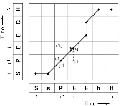
Those three transitions are illustrated in Figure 1, where T is interpreted as a Test sentence compared with the some reference templates R.

Therefore, the problem of DTW is to minimize, Dist (D), is the same as Forward Dynamic Programming of deterministic shortest path algorithm [9]. Therefore it can be converted from (ordinary) backward to forward, and can be modelled as a finite state system.

B. One dimension DTW

(3)

Volume 2, Issue 6, November-December-2017 | www.ijsrcseit.com | UGC Approved Journal [ Journal No : 64718 ] 2. Continuity – the path advances increasingly, step by

step; indices i and j add to by maximum 1 unit on a step.

3. Boundary – the path begins from left-down corner and ends with right-up corner [21].

Figure1. A sample line graph for DTW

C. Two Dimensional DTW

Extending the Dynamic Time Warping method to two dimensions is not a simple task. The input data is no longer a 1-dimensional series but rather a 2-dimensional matrix. This matrix can represent images or any other 2-dimensional data. A two dimensional dynamic warping algorithm could be used for a variety of applications such as text and facial recognition and is described as a fundamental technique for pattern recognition Various algorithms have been proposed to solve the problem. Solution are proposed in [16, 17] but both unfortunately exhibit exponential time complexity. It is shown in [18] that the 2-dimensional warping problem is NP-complete. Approximation methods have been described in [19]. A polynomial-time and supposedly accurate algorithm for 2D warping based on DTW is proposed in [20]. This algorithm, its improvement, extension, and testing are the subjects of the rest of this report. The result of 2D-DTW were showed in the table 3.

i. Preprocessing

The speech signal is decomposed into a sequence of overlapping frames. The frame size of 25 ms and 10ms frame shift is used for the analysis of speech signal. The input speech data are pre emphasized with co-efficient of 0.97 using a first order digital filter. The samples are weighted by a Hamming window for avoiding spectral distortions. The resulting windowed

frames are used to extract both features MFCC and LPCC. The result of 1-DTW showed in the table 2.

ii. MFCC

Figure 2 shows block diagram of extraction of MFCC feature from a signal.

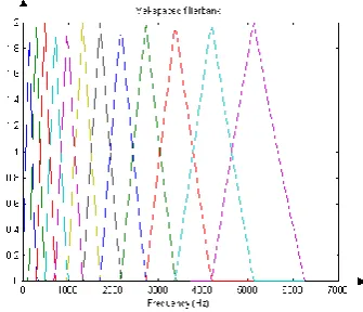
Figure 2. Block diagram for the feature extraction process of MFCC

Mel Filter Bank is use to determine the frequency con-tent across each filter. The Mel filter bank is built from triangular filters. The filters are overlapped in such a way that the lower boundary of one filter is situated at the center frequency of the next filter. 1000 Hz was defined as 1000mels. An approximate formula to compute the Mels for a given frequency in Hz is using equation 3 [8].

( ) [ [ ]] (3)

We are just inspired by generally how much vitality happens at each spot. Here an arrangement of 26 triangular filters are taken. To compute channel bank energies we increase each channel keep money with the energy range, and after that include the coefficients. Once this is performed we are left with 26 numbers that give us an sign of how much energy was in each filter bank. Discrete Cosine Transform (DCT) takes after logarithm for these 26 energy values. DCT is ascertained utilizing condition appeared in equation 4.

(4)

Figure 3. A Mel Frequency Scale

The overlapping windows in the frequency domain can be directly used. The energy within each triangular window is obtained and followed by the DCT to achieve better compaction within a small number of coefficients and results are known as MFCC. The data will be stored in the database and take to compare with the voice input at the testing phase with same steps of process.

First and derivative coefficients are calculated for each frame as given in equations 5 and 6.

[ ] [ ] [ ] (5)

[ ] [ ] [ ] (6)

iii. LPCC

Let assessing the fundamental parameters of a speech signal, LPCC has turned out to be one of the perdominant methods. . The essential subject behind this strategy is that one speech sample at the current time can be predicted as a linear combination of past speech samples. Algorithm for LPCC is appeared in Figure 3.

The first phase of the algorithm is pre-processing. After pre-preprocessing, the speech signal is subdivided into frames. This process is the same as multiplying the entire speech sequence by a windowing function. The windowing process to be completed means move on to next phase. The next phase is Linear Predictive Analysis (LPA). LPA is grounded on the theory, that the shape of the vocal tract chooses the character of the sound being delivered. A computerized all-post channel is utilized to demonstrate the vocal tract and has a move work spoke to in z area as in equation 7.

Figure 4. Block diagram for the feature extraction process of LPCC

( )

∑

(7)

where V(z) is the vocal tract transfer work. G is the gain of the filter, {ak}is a the set of auto regression

coefficients known Linear Prediction Coefficients (LPC), p is the request of the all-pole filter. One of the efficient techniques for assessing the LPC coefficients and the filter gain is Autocorrelation technique [10]. Last phase of this algorithm is cepstral analysis, which refers to the process of finding the cepstrum of speech sequence. Fundamentally, there are two types of cepstral approaches: FFT cepstrum and LPC cepstrum. In the previous case the real cepstrum is characterized as the backwards FFT transform of the logarithm of the speech size range characterized by following equation 8.

̂[ ]

∫ [ ( )]

(8)

Where and demonstrates the Fourier spectrum of a signal and cepstrum separately [11]. Be that as it may, one more method for evaluating these cepstral coefficients is from the LPC by means of a set of recursive technique and the coefficients in this way acquired are known as straight Linear prediction cepstral coefficients (LPCC).

iv. Stochastic DTW

Juang [12] presented stochastic dynamic time warping method for speaker independent recognition, which combines a standard dynamic time warping method with a Hidden Markov model [13]. Let S and A be the state sequence and observed sequence, O (s1,, s2,.. si; oj)

(5)

Volume 2, Issue 6, November-December-2017 | www.ijsrcseit.com | UGC Approved Journal [ Journal No : 64718 ]

IV. RESULTS AND DISCUSSION

A. Data

Commands words uttered in English are recorded with the help of a unidirectional microphone in a calm environment is considered as data set. Data are recorded using a recording tool audacity in a closed room. The sampling rate used for recording is 16 kHz. The description about the data used is also given in Table I.

Table I. Results of DTW With Eight Command Words

S.No Uttered words

Sample words duration time(ms)

No. Of Samples

1 Start 0.0627 10031

2 Left 0.0929 14861

3 Right 0.0579 9845

4 Forward 0.0685 10959 5 Backward 0.0679 13375

6 Up 0.0522 8359

7 Down 0.0418 5699

8 Stop 0.0114 8916

Table II. Results of 1-DTW with Eight Command Words

Start Left Right Forward Backward Up Down Stop

Start 0 30.5988 22.0397 66.7249 33.5013 29.6243 54.2266 68.0698

Left 30.5988 0 26.5723 89.9319 46.888 39.8305 78.2258 89.9042

Right 22.0397 26.5723 0 75.5159 37.5828 34.5234 63.7876 80.6848

Forward 66.7249 89.9319 75.5159 0 54.4777 74.299 58.9084 77.4254

Backward 33.5013 46.8808 37.828 54.477 0 44.8455 54.2266 71.3358

Up 29.6243 39.8305 34.5234 74.2499 44.8455 0 51.7068 57.1259

Down 54.9527 78.2258 63.7876 58.4084 54.2266 51.7068 0 47.1963

Stop 68.0698 89.9042 80.6848 77.4254 71.3358 57.1259 47.1963 0

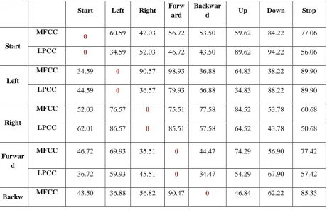
Table III. Results of 2D-DTW with Eight-Command Word Tested with MFCC

Start Left Right Forw

ard

Backwar

d Up Down Stop

Start

MFCC

0 60.59 42.03 56.72 53.50 59.62 84.22 77.06

LPCC ₀ _34.59 _52.03 _46.72 _43.50 _89.62 _94.22 _56.06

Left

MFCC 34.59 0 90.57 98.93 36.88 64.83 38.22 89.90

LPCC 44.59 0 36.57 79.93 66.88 34.83 88.22 89.90

Right

MFCC 52.03 76.57 0 75.51 77.58 84.52 53.78 60.68

LPCC 62.01 86.57 0 85.51 57.58 64.52 43.78 50.68

Forwar d

MFCC 46.72 69.93 35.51 0 44.47 74.29 56.90 77.42

LPCC 36.72 59.93 45.51 0 34.47 54.29 67.90 57.42

(6)

ard LPCC 34.50 46.88 45.82 89.47 0 35.84 83.22 71.33

Up

MFCC 79.62 72.83 54.52 34.24 54.84 0 81.70 32.12

LPCC 49.62 63.83 74.52 74.24 34.84 0 89.70 78.12

Down

MFCC 74.95 68.22 23.78 28.40 34.22 61.70 0 98.19

LPCC 84.95 98.22 33.78 48.40 84.2 62.70 0 67.19

Stop

MFCC 28.06 49.90 30.68 57.4 71.33 37.12 37.19 0

LPCC 48.06 59.90 70.68 67.42 41.33 27.12 67.19 0

V.

CONCLUSION

Speech data were analyzed using DTW. One dimensional speech template of eight command words were considered and taken for evaluation. MFCC and LPCC features of the same set of speech data are extracted, DTW is applied, and then the results were analyzed. Future work should prioritize methods to reduce the computation load and improve the computing speed by optimizing the implementation of the DTW algorithm, and should explore hierarchical or classification techniques to minimize the number of possible matches.

VI. REFERENCES

[1]. Palden Lama and Mounika Namburu. Speech Recognition with Dynamic Time Warping using MATLAB”, CS 525, SPRING 2010 – PROJECT REPORT.

[2]. Chunsheng Fang. From Dynamic Time Warping (DTW) to Hidden Markov Model (HMM), 2009/3/19,Final project report for ECE742 Stochastic Decision.

[3]. Stan Salvador and Philip Chan. FastDTW: Toward Accurate Dynamic Time Warping in Linear Time and Space

[4]. E- Hocine Bourouba. Mouldi Bedda and Rafik Djemili, Isolated Words Recognition System Based on Hybrid Approach DTW/GHMM, Informatica 30 (2006) 373–384 373.

[5]. Rashid R.A and Mahalin N.H and Sarijari M.A and Abdul Aziz A.A. Security system using

biometric technology: design and implementation of Voice Recognition System (VRS),International Conference on Computer and Communication Engineering, 2008.

[6]. L.Muda and K.M Begam and I. Elamvazuthi. Voice recognition algo¬rithms using Mel Frequency Cepstral Coefficient (MFCC) and Dynamic Time Warping (DTW) techniques, Journal of Computing, 2010, 2(3):138–143. [7]. DAVIS, S. & MERMELSTEIN, P. 1980.

Comparison of parametric representations for monosyllabic word recognition in continuously spoken sentences. Acoustics,Speech and Signal Processing,IEEE Transactions on, 28, 357-366. [8]. Bhadragiri Jagan Mohan, Ramesh Babu. N,

Speech Recognition using MFCC and DTW, https://www.researchgate.net/publication/260762 671, DOI: 10.1109/ICAEE.2014.6838564. [9]. L.Muda and K.M Begam and I. Elamvazuthi.

Voice recognition algo¬rithms using Mel Frequency Cepstral Coefficient (MFCC) and Dynamic Time Warping (DTW) techniques, Journal of Computing, 2010, 2(3):138–143 [10]. Octavian, C., Abdulla, W. and Zoran, S. 2005,

Performance Evaluation of Front-end Processing for Speech Recognition Systems.

[11]. Rabiner, L.R., Shafer, R.W. 2009, Digital Processing of Speech Signals, 3rd edition, Pearson education in south Asia.

(7)

Volume 2, Issue 6, November-December-2017 | www.ijsrcseit.com | UGC Approved Journal [ Journal No : 64718 ] [13]. S Nakagawa, Speaker-independent phoneme

recognition in continuous speech by a statistical method and a stochastic dynamic time warping method, Tech Report CMU-CS-86-102, Carnegie Mellon University, 1985.

[14]. Octavian Cheng, Waleed Abdulla, Zoran Salcic Performance Evaluation of Front-end Processingfor Speech Recognition Systems School, 2005.

[15]. Veton Kepuska. Speech Processing Project Linear Predictive coding using Voice excited Vecoder, ECE 5525, Osama Saraireh, Fall 2005. [16]. T. Levin and R. Pieraccini. Dynamic planar

warping for optical character recognition. IEEE, International Conference on Acoustics, Speech, and Signal Processing, 3:149–152, 1992. [17]. S. Uchida and H. Sakoe. A monotonic and

continuous two-dimensional warping based on dynamic programming. In Proc. 14th International Conference on Pattern Recognition, volume 1, pages 521–524, 1998.

[18]. Daniel Keysers and Walter Unger. Elastic image matching is np-complete. Pattern Recogn. Lett., 24(1-3):445–453, 2003

[19]. S. Uchida and H. Sakoe. An approximation algorithm for two-dimensional warping, Institute of Electronics, Information, and Communication Engineers Transactions on Information & Systems, E83-D(1):109–111, 2000.

[20]. H. Lei and V. Govindaraju. Direct image matching by dynamic warping. In Proc. of the 1st IEEE Workshop on Face Processing in Video, In conjunction with the IEEE International Conference on Computer Vision and Pattern Recognition (CVPR’04), Washington D.C., 2004.