The Late Quaternary Paleolimnology of Lake Ontario

(1)

Western University Western University

Scholarship@Western

Electronic Thesis and Dissertation Repository

9-4-2014 12:00 AM

The Late Quaternary Paleolimnology of Lake Ontario

Ryan Hladyniuk

The University of Western Ontario

Supervisor

Dr. Fred J. Longstaffe

The University of Western Ontario Graduate Program in Geology

A thesis submitted in partial fulfillment of the requirements for the degree in Doctor of Philosophy

Follow this and additional works at: https://ir.lib.uwo.ca/etd

Part of the Geochemistry Commons

Recommended Citation Recommended Citation

Hladyniuk, Ryan, "The Late Quaternary Paleolimnology of Lake Ontario" (2014). Electronic Thesis and Dissertation Repository. 2401.

https://ir.lib.uwo.ca/etd/2401

(2)

THE LATE QUATERNARY PALEOLIMNOLOGY OF LAKE ONTARIO

(Thesis format: Integrated Article)

by

Ryan Hladyniuk

Graduate Program in Earth Sciences

A thesis submitted in partial fulfillment of the requirements for the degree of

Doctor of Philosophy

The School of Graduate and Postdoctoral Studies The University of Western Ontario

London, Ontario, Canada

(3)

Abstract

(4)

iii

Keywords

(5)

Epigraph

Meltwaters did rush to the sea They say – from Lake Agassiz

And that made it cold We are constantly told

But the pathways aren’t shown to me!

(6)

v

Dedication

This thesis is dedicated to my parents, Zeferina and Peter Hladyniuk.

(7)

Acknowledgments

He who tops the list of acknowledgments is my supervisor Fred Longstaffe. Throughout the past 6 years, Fred has exemplified what it is to be a great supervisor. He offers creative academic ideas, encouragement towards research, virtually limitless patience and the ability to extend your mind in areas you never thought possible. Fred is also an excellent role model; his leadership has advanced my personal professional development skills while maintaining the highest ethical (academic and personal) integrity. Without Fred, I would not have been able to participate in the numerous conferences and field trips I attended. In addition, I would have not been a member of such a prestigious group of international and governmental collaborators. In my first meeting with Fred, Fred asked me; “What do you know about lake sediment cores?” I replied; “All I know is that they are round.” Getting your first question wrong (sediment cores are cylindrical) does not leave a particularly good first impression; however, Fred remained confident in my abilities then, as much as he does now. I can say with confidence, that without Fred I would not have progressed to be the scholar I am today. Fred, thank you for all that you have provided me (skills, life lessons and countless delicious ‘feedings’). I am extremely honoured to have you as a supervisor –I am also grateful to call you my friend.

I also thank Allan Crowe (Canada Centre for Inland Waters, Environment Canada) for facilitating core sampling, and the captain and crew of the Canadian Coast Guard Ship Limnos for core collection –ultimately the foundation for my Ph.D. project. Also at Canada Centre for Inland Waters, I thank Christina Jaskot, Brian Trapp and Ian Droppo for allowing me to obtain grain-size measurements in their laboratory. I sincerely thank Francine

McCarthy (Brock University) for welcoming me into her lab and teaching me the skills to extract pollen from lake sediments. In addition, I thank Francine for allowing me to attend her wonderful course on palynology. I am grateful to John King and staff (University of Rhode Island, Graduate School of Oceanography) for providing sediment core images and the University of Arizona (AMS laboratory) for radiocarbon dates.

(8)

vii

Lewis) for their thoughtful revisions and skillful questions during my defense. All of you have greatly advanced this work.

Much of the analytical work would not be possible without the assistance of the staff of the Laboratory for Stable Isotope Science (The University of Western Ontario). I appreciate the time and patience offered by Kim Law, Grace Yau, and Li Huang. All of you have greatly advanced my technical skills in the field of stable isotope mass spectrometry and I thank you for that. I would also like to thank my laboratory and university colleagues that have

provided helpful insight toward project design and assistance on experiments: Rebecca Macdonald, Ayumi Hyodo, Sam Russel, Duane Petts, Jessica Metcalfe, Beth Hundey, Natasha Bumstead, Nicolle Bellissimo, Christine Cizkowski, Nadine Wakabayashi, Paul Szpak, Scott Colborne, Farnoush Tahmasebi, Laura Sanchez and Nelson Cho.

A special ‘thank you’ is needed for; (i) Avner Ayalon (Geological Survey of Israel) for

enhancing my critical thinking skills in the field of isotope science, (ii) Mike Lewis (Geological Survey of Canada), ‘the godfather’ of Great Lakes research, for the many

delightful and constructive talks about limnology in general and (iii) Nadia Dildar for coaching me through the process of lipid extraction and n-alkane measurements.

The project would not be possible without funding. Operating funds were provided by a Natural Sciences and Engineering Research Council of Canada Discovery Grant (FJL) and an Ontario Graduate Scholarship (RH). Infrastructure support was provided by the Canada Foundation for Innovation and the Ontario Research Fund (FJL). The research was also made possible in part through additional research time provided through the Canada Research Chairs program. I also wish to express my gratitude toward the donors and organizations of the many scholarships I obtained; Robert and Ruth Lumsden Award, Graduate Thesis Research Award, Robert Hodder Travel Bursary, Kenneth N. Weaver Student Travel Award (Geological Society of America, North-eastern section), Geological Society of America Student Travel Award (North-central section), and the International Association for Great Lakes Research-Ontario Ministry of Natural Resources Student Travel Award.

(9)

have had together, especially the RRBD faithful (a short list of friends in no particular order): Carter Hutton, Billy Boquist, Mike and Kelly Sellan, Chris Unick, Adam Fron, Justin

Everett, Troy Prezio, Brent Irwin, Steve Hosegood, Kevin Britton, Ryan Baird, Jeff Coull, Kory McEwan, Derrick Hosanna, Adam and Michelle Nemeth, Adam Fabiano, Brad and Nicole Yeo, Mark Davis, Peter Franchin, Kyle Lamb, Keyvan Hunt, Randy and Janelle Hanagan and the list goes on!

Thank you to the Andrews family for operating the Komoka Classics Senior ‘AA’ hockey

club (formerly Lucan-Ilderton Jets) and allowing me to play for such a first class

organization. I also thank my hockey teammates, coaches and trainers over the years (the list is long).

Last, but certainly not least, my family to whom I owe everything. Above all, I thank my parents Zeferina and Peter Hladyniuk for encouraging me to chase my dreams and make my university ‘career’ a reality. I had infinite support (both financial and emotional) from the

best role models a son could ask for, thank you. I truly would not be the person I am today without Zef and Pete. In addition to thanking my parents, I would like to acknowledge my brother Nik Hladyniuk. He has always kept me ‘in-line’, as any big brother would, and has

provided our family with countless hours of humour. Above all, he provides limitless enthusiasm towards my academic success and only thinks of the positive outcomes with respect to my goals. To my wife Melissa, I thank you for listening to my long-winded scientific problems and for constantly supporting my quest for knowledge. You are always there when I need you the most, thank you. I also appreciate Tatem and Hope for giving me the chance to live a well-rounded, family life. To my future son or daughter, thank you for the many kicks and the wave you gave me in the ultrasound; I cannot wait to meet you, hope this thesis makes you proud. I also have to mention my late Babcia and Dziadzia, they would have been proud to see this day and I miss them very much. Concluding, I have to thank the Kondakow’s (Mickey, Louise, Megan and especially Mike for all the PYT concerts), the

(10)

ix

List of Tables

Table 2.1. Radiocarbon dates were obtained at the University of Arizona AMS Laboratory in

Tuscon, AZ, USA. The date for the Pisidium sp. clam shells was corrected for the hard water effect (HWE) by subtracting 535 ± 15 years (Anderson and Lewis, 2012) prior to converting it to a calibrated age. Radiocarbon dates were converted to calibrated ages using the

computer program CLAM and INTCAL09 (Reimer et al., 2009; Blaauw, 2010). Calibrated ages represent the midpoint of the sampled interval; C1334 545 cm, C1335 525 cm and C1336 425 cm. ... 29

Table 4.1. Abundances of n-alkanes in Lake Ontario Core 1336, reported in absolute (μg/g)

and relative abundances (%) (C35 is omitted) by depth (meters) and age (calibrated years BP). Bold and italicized values represent the highest n-alkane abundance for a given sample. .. 112

Table 4.2. Carbon-isotope compositions (VPDB, ‰) of n-alkanes in Lake Ontario Core

(15)

List of Figures

Figure 1.1. Satellite maps of the Laurentian Great Lakes (red circle). Figure modified from

Google maps (http://www.google.com/maps). ... 2

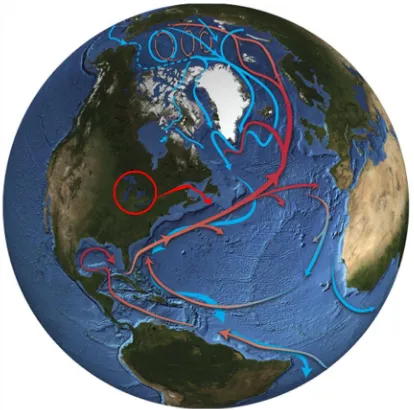
Figure 1.2. Thermohaline circulation (THC) in the Atlantic and Arctic Oceans. Warmer

surface currents (red) and colder deep currents (blue) strongly influence Earth’s climate. The

Great Lakes (circled red) presently drain northeastward (red arrow) into the Atlantic Ocean at a critical location where the warm current transports heat (and salt) northward into the Nordic seas between Greenland and Norway and the Labrador Sea where convection processes (THC) occur. The northward-flowing warm surface current and returning deep cold current constitute the Atlantic Meridional Overturning Circulation (AMOC). Rapid outflows of freshwater from impoundments of meltwater during deglaciation of North America are thought to have diluted the warm salty surface current sufficiently to prevent sinkage

(convection) during winter cooling in the north Atlantic and to have slowed THC and AMOC ~12,900-11,500 cal BP. The slowdown in convection is thought to have diverted the warm current eastward, thereby slowing northward transport of heat and inducing the YD cold event. Figure modified from Dickson and Dye (2007). ... 5

Figure 1.3. Maximum extent (~24,000 cal [20,000 14C] BP) of the Laurentide Ice Sheet

(LIS) in North America. The Great Lakes are circled in red. Figure modified from the National Science Foundation website (http://www.nsf.gov). ... 7

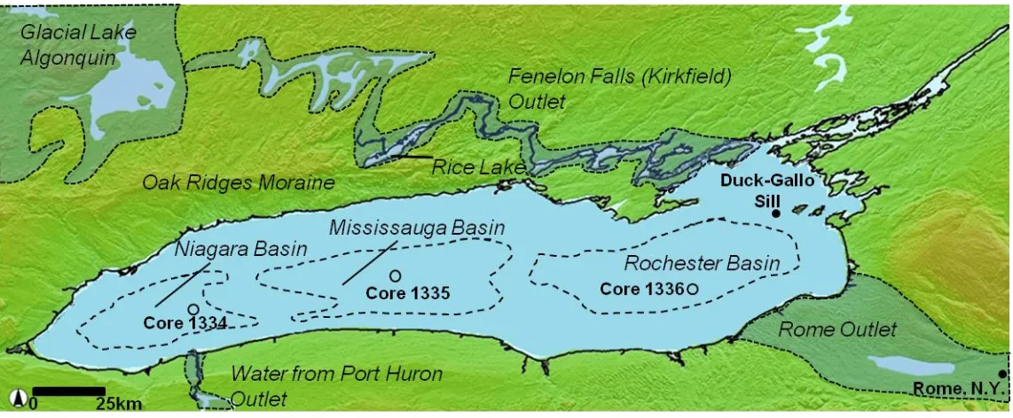
Figure 1.4. DEM of Lake Ontario. Core locations are denoted by circles and labeled

respectively. Figure modified from the National Oceanic and Atmospheric Administration data center website (http://ngdc.noaa.gov/mgg/dem/). ... 13

Figure 1.5. Geological map of southern Ontario. The yellow line defines the boundary

between Paleozoic carbonates (to the southwest) and Precambrian bedrock (to the north). Lake Ontario’s watershed contains both types of regional geology. Figure modified from

(16)

xv

Figure 2.1. Digital Elevation Model (DEM) of the Great Lakes basin. Important outlets and

locations are labeled. Figure modified from the National Oceanic and Atmospheric

Administration data center website (http://ngdc.noaa.gov/mgg/dem/). ... 20

Figure 2.2. DEM Lake Ontario region showing the locations of sediment piston cores: Core

1334 (43 24’ 23” N and 79 00’ 05” W; water depth, 110.3 m; core length, 17.00 m), Core 1335 (43 33’ 19” N and 78 09’ 01” W; water depth, 192 m; core length, 18.20 m), Core 1336 (43 30’ 28” N and 76 53’ 07” W; water depth, 221.5 m; core length, 18.41 m). Several locations discussed in the text are also shown. Figure modified from the National Oceanic and Atmospheric Administration data center website

(http://ngdc.noaa.gov/mgg/dem/). ... 25

Figure 2.3. Photographs of: a) Fabaeformiscandona caudata, b) Candona subtrigangulata

and c) Pisidium species clams... 26

Figure 2.4. Generalized lithology of the Lake Ontario sediments in Cores 1334, 1335 and

1336. Locations of radiocarbon-dated material are denoted by stars. ... 30

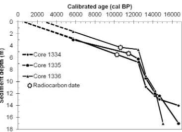
Figure 2.5. Non-Bayesian, linear interpolated, age-depth produced by CLAM (Blaauw,

2010). All radiocarbon dates were converted to calibrated ages by CLAM using INTCAL09 (Reimer et al., 2009). Three radiocarbon dates were used along with results from previous studies on Lake Ontario to establish the age-depth profiles (Schroeder and Bada, 1978; Carmichael et al., 1990; Hutchinson et al., 1993; McAndrews, 1994; Pippert et al., 1996; Silliman et al., 1996; Anderson and Lewis, 2012). See Table 2.1 for details. ... 31

Figure 2.6. Data for Core 1334: (a) median grain size; (b) mineralogy (red line, feldspars;

(17)

Figure 2.7. Data for Core 1335: (a) median grain size; (b) mineralogy (red line, feldspars; blue line, clays; green line, carbonates; black line, quartz) (c) ostracode abundances, valves per gram sediment (v/g), and (d) δ18Olakewater values inferred from ostracode valves and clam shells. Gray shaded area indicates a renewedperiod of glacial meltwater influx. Divisions between sediment units are denoted by continuous solid lines across (a), (b), (c) and (d). Biostratigraphic zonations are illustrated by braces in (c). Post-glacial isotopic changes are demarcated by solid lines that divide (d) and are placed at 10,500, 8,300 and 6,800 cal BP. 33

Figure 2.8. Data for Core 1336: (a) median grain size; (b) mineralogy (red line, feldspars;

blue line, clays; green line, carbonates; black line, quartz) (c) ostracode abundances, valves per gram sediment (v/g), and (d) δ18Olakewater values inferred from ostracode valves and clam shells. Gray shaded area indicates a renewedperiod of glacial meltwater influx. Divisions between sediment units are denoted by continuous solid lines across (a), (b), (c) and (d). Biostratigraphic zonations are illustrated by braces in (c). Post-glacial isotopic changes are demarcated by solid lines that divide (d) and are placed at 10,500, 8,300 and 6,800 cal BP. 34

Figure 2.9. (a) Three-point running average of δ18Olakewater values for Cores 1334, 1335, and

1336. (b) Ostracode valve and clam shell oxygen isotope compositions (VPDB) (vital effect corrected, subtract 2.2 ‰ from VPDB data) for Lake Ontario. Red and blue dots represent Champlain valley Candona record from Beekmantown 1 and 2 cores, as outlined by Cronin et al. (2012). A generalized age for the Beekmantown cores was inferred from Rayburn et al. (2011). (c) Champlain Valley stratigraphy outlined by Cronin et al. (2012). ... 47

Figure 2.10. (a) GISP2 oxygen-isotope record illustrating the Younger Dryas event (Yu and

Eicher, 1998). (b) Three-point running average of δ18Olakewater values for Cores 1334, 1335 and 1336. Gray shaded area indicates the period of the terminal glacial meltwater influx at 13,000-12,500 cal [11,100-10,500 14C] BP. ... 48

Figure 2.11. Lake elevation versus age in the main Ontario basin, as outlined by Anderson

(18)

xvii

Figure 3.1. Digital Elevation Model (DEM) of the Great Lakes basin. Important outlets and

locations are denoted in italics. Figure modified from the Nation Oceanic and Atmospheric Administration data center website (http://ngdc.noaa.gov/mgg/dem/). ... 62

Figure 3.2. Carbon isotope systematics and sources of DIC to Lake Ontario. Figure

modified from Meyers and Teranes (2001). ... 65

Figure 3.3. DEM Lake Ontario region showing the locations of sediment piston cores: Core

1334 (43 24’ 23” N and 79 00’ 05” W; water depth, 110.3 m; core length, 17.00 m), Core 1335 (43 33’ 19” N and 78 09’ 01” W; water depth, 192 m; core length, 18.20 m), Core 1336 (43 30’ 28” N and 76 53’ 07” W; water depth, 221.5 m; core length, 18.41 m). Several locations discussed in the text are also shown. Figure modified from the National Oceanic and Atmospheric Administration data center website

Figure 3.4. Non-Bayesian, linear interpolated, age-depth model for Cores 1334, 1335 and

1336 produced using CLAM (Blaauw, 2010). All radiocarbon dates were converted to calibrated ages by CLAM using INTCAL09 (Reimer et al., 2009). Three radiocarbon dates were used along with additional information from previous studies on Lake Ontario to establish the chronology (Schroeder and Bada, 1978; Carmichael et al., 1990; Hutchinson et al., 1993; McAndrews, 1994; Pippert et al., 1996; Silliman et al., 1996; Anderson and Lewis, 2012). ... 70

Figure 3.5. Ostracode valve and clam shell carbon isotope compositions for the period

~16,000 to 6,000 cal BP. ... 75

Figure 3.6. Carbon mass accumulation rates, nitrogen mass accumulation rates and C/N

ratios for Core 1334. ... 77

ratios for Core 1335. ... 78

(19)

Figure 3.9. Bulk sediment organic matter carbon isotope compositions Cores 1334, 1335 and 1336. ... 81

Figure 3.10. Bulk sediment organic matter nitrogen isotope compositions for Cores 1334,

1335 and 1336 ... 82

Figure 3.11. DEM overlain by the LIS margin and glacial lakes in the Great Lakes basin: (a)

Mackinaw Interstadial from 16,000 to 15,300 cal BP. Drainage of Lake Ypsilanti is indicated by the arrow; (b) Ice readvance from 15,300 to 14,500 cal BP. Lake Whittlesey drainage is indicated by the arrow. ... 85

Figure 3.11 (continued). DEM overlain by the LIS margin and glacial lakes in the Great

Lakes basin: c) Rise of glacial Lake Iroquois from 14,500 to 13,000 cal BP. Drainage into glacial Lake Iroquois from glacial Lake Algonquin is indicated by the arrow. Water from Erie basin did not enter the Ontario basin at this time; (d) Fall of glacial Lake Iroquois and formation of early Lake Ontario from 13,000 to 12,500 cal BP. Drainage into Lake Ontario occurred through both active outlets of glacial Lake Algonquin as indicated by the arrows. Increased meltwater supply inhibited the marine invasion of the Champlain Sea into the Ontario basin. Figures adapted from Lewis et al. (1994), Calkin and Feenstra (1985), Karrow (1989) and the National Oceanic and Atmospheric Administration data center website

(http://ngdc.noaa.gov/mgg/dem/)...86

Figure 4.1. Digital elevations model (DEM) of Lake Ontario region showing the location of

sediment piston Core 1336 obtained by the CCGS Limnos in July 2008: 43 30’ 28” N and 76 53’ 07” W; water depth, 221.5 m; core length, 18.41 m. Figure modified from the National Oceanic and Atmospheric Administration data center website

Figure 4.2. Non-Bayesian, linear interpolated age-depth model for Core 1336 produced by

(20)

xix

Figure 4.3. Gas chromatograms for the non-polar lipid fraction from Core 1336 sediments.

Molecular weights of odd-chain n-alkanes and the internal standard (I.S.) 5α-androstane are annotated. (a) Typical chromatogram for post-glacial sediments. (b) Typical chromatogram for glacial sediments. ... 113

Figure 4.4. (a) Average chain length of n-alkanes calculated using ACL = (ΣCn•n)/(ΣCn),

where Cn is the concentration of n-alkane containing n carbon atoms (Chikaraishi and Naraoka, 2003). (b) The terrestrial to aquatic (TAR) n-alkane ratio was calculated using TAR= (C27+C29+C31)/(C17+C19+C21), adapted from Silliman et al. (1996). (c) n-Alkane mass accumulation rates (MARs) calculated using MARs= concentration of total n-alkanes • linear sedimentation rates • dry bulk density • 10-6

... 114

Figure 4.5. Standard n-alkane chain-length distributions for various time intervals. The

average relative abundance for a given time interval is represented by the height of the individual column and the standard deviation is shown by error bars. The general

distribution for each time interval is shown by the red trace above the bar graph. ... 116

Figure 4.6. The n-alkane relative abundances (%) organized by sediment age (cal BP). The

abundances of n-alkanes are divided into short-, mid-, and long-chain lengths for easier comparison within a group. ... 117

Figure 4.7. Age (cal BP) versus δ13C values for each n-alkane. ... 120

Figure 4.8. Pollen diagram for Rostock mammoth site (redrawn from McAndrews, 1994).

See Figure 1 for location. Pollen zone 1p represents a polar desert. The high abundances of spruce and pine pollen likely represent recycled pollen grains. A transition from tundra woodland to boreal woodland occurs in pollen zone 1a. A pine-dominated forest was established at ~12,900 cal BP. Red arrows indicate the timing of increased abundances of birch and willow pollen. ... 122

Figure 4.9. Schematic diagram illustrating potential sources of OM entering ancient Lake

(21)

included recycled and degraded terrestrial vegetation. (b) During formation of glacial Lake Iroquois, aquatic macrophytes were the major source of OM in lake sediments. Sphagnum mosses were likely less important. ... 125

Figure 4.9 (continued). (c) Lower lake levels of post-glacial Lake Iroquois were associated

with increased abundances of algal biomarkers (C17, C19); hydrologic closure also favoured growth of aquatic macrophytes. There was also some OM contribution from the coniferous-forested watershed to the lake sediments. (d) Increased precipitation caused Lake Ontario to rise. The forested watershed, now dominated by angiosperms, was a major contributor to the lake sediment OM record, particularly through drowned shorelines. OM contributions from algal and aquatic macrophytes continued to be significant.………..126

Figure 4.10. Roblin Lake pollen record, as adapted from Terasmae (1980) and re-drawn for

(22)

xxi

List of Appendices

Appendix I provides digital images of each core (Core 1334; Niagara basin, Core 1335;

Mississauga basin, and Core 1336; Rochester basin), divided into ~1 m intervals. Core descriptions include general commentary, grain-size measurements, Munsell Soil Colour Charts (2000) classifications and correlations to other studies (Hutchinson et al., 1993; Pippert et al., 1996). ... 153

Appendix II reports the results obtained for isotopic and elemental standards. ... 206

Appendix III describes the sediment depths and age of grain-size measurements obtained.

... 213

Appendix IV reports the mineralogy for each core as determined by powder X-Ray

diffraction. ... 215

Appendix V ostracode valves and clam shells carbon and oxygen-isotopic compositions.

Calculated lakewater oxygen-isotope compositions are also reported. ... 221

Appendix VI bulk organic matter carbon and nitrogen elemental and isotopic compositions.

Calculated molar carbon to nitrogen ratios are also reported. ... 229

Appendix VII reports the n-alkane abundances and carbon isotopic compositions. ... 232

Appendix VIII provides the gas-chromatograph spectrums used to calculate n-alkane

(23)

1

Chapter 1

1 Introduction

1.1 Overview

The glacial history of the Laurentian Great Lakes (Fig. 1.1), and its relationship to global climatic and environmental changes, have been studied since the early 1900s. In

particular, it has been suggested that meltwater from the ablating Laurentide Ice Sheet (LIS) was routed through the Great Lakes to the Atlantic Ocean, weakening thermohaline circulation (THC) in the Atlantic Meridional Overturning Circulation (AMOC) and triggering the Younger Dryas (YD) cooling event at ~12,900 cal [11,020 14C] BP (Teller, 1985; Broecker et al., 1989; Teller, 1990; Teller, 1995). This proposed history has been the subject of considerable debate over the past several decades (Fritz et al., 1975; Lewis et al., 1994; Rea et al., 1994; Fisher and Lowell, 2006; Cronin et al., 2008; Fisher et al., 2009; Murton et al., 2010; Teller, 2013). As such, there remains much to be investigated in the Great Lakes region to determine the specific timing and extent of meltwater contributions to each lake. The presence of glacial meltwater in the Great Lakes can be identified using proxies such as the oxygen isotopic composition of shelly fauna preserved in lake sediments. Lake Ontario – the focus of this thesis – is located at the end of the Great Lakes chain-of-lakes, and hence provides a unique opportunity to pinpoint meltwater passage from the lower Great Lakes to the Atlantic Ocean.

Lake Ontario sediments also contain organic matter (OM) proxies that offer an

(24)

2

Figure 1.1. Satellite maps of the Laurentian Great Lakes (red circle). Figure modified from Google maps

(25)

3

Lake Ontario to return to overflow conditions at ~8,300 cal [7,500 14C] BP (Edwards et al., 1996; Anderson and Lewis, 2012). Continual warming and still wetter conditions developed by ~6,800 cal BP and with the return of upper Great Lakes drainage during the Nipissing rise at ~5,800 cal BP, Lake Ontario water levels rose abruptly by ~10 m, followed by a more gradual increase to near present levels by 3,000 cal [2,890 14C] BP (Edwards et al., 1996; Anderson and Lewis, 2012). Lake Ontario’s

ecological/environmental response to these shifting climatic conditions and water levels, as recorded in OM, has been examined in only a few previous studies (Silliman et al., 1996; McFadden et al., 2004; 2005). A more detailed historical baseline for Lake Ontario’s response to changing climatic conditions should provide a useful frame of

reference for anticipating the consequences of future climate change. In particular, OM in Lake Ontario sediments should contain a biochemical record of (i) its source (e.g., terrestrial or lacustrine), (ii) changes in primary production within the lake, and (iii) variations in allochthonous versus autochthonous OM contributions in response to shifting environmental conditions.

Previous studies on bulk chemical and isotopic analysis of OM by itself, however, is not always suitable for discrimination among the types of OM present, or its terrestrial versus lacustrine sources, especially in glacio-lacustrine deposits (Hyodo and Longstaffe, 2011). A multi-proxy approach, combining compound-specific measurements of lipid

biomarkers such as n-alkanes with more traditional bulk OM analysis, allows for more accurate assessment of primary lacustrine productivity and terrestrial allochthonous inputs. A few previous studies of Lake Ontario have begun such work (Silliman et al., 1996; McFadden et al., 2004; 2005), and that approach is expanded upon here.

1.2 Research questions

(26)

4

order to identify changes in lacustrine productivity versus terrestrial OM inputs under varying environmental conditions – within the broader framework of regional and global climate change. One part of this thesis determines the timing and extent of glacial meltwater movement through Lake Ontario. As mentioned earlier, discharge to the Atlantic Ocean from glacial Lake Agassiz and other large proglacial lakes via the Great Lakes is posited to have disrupted THC (Fig. 1.2) and caused the YD (Broecker et al., 1989). More recent research, however, suggests that the meltwater entered the Arctic Ocean mostly through a northwestern outlet (Murton et al., 2010). Still other researchers suggest that Glacial Lake Agassiz evaporated rather than drained into either ocean (Fisher and Lowell, 2012; Lowell et al., 2013). Within this conceptual context, the timing and extent of glacial meltwater input into Lake Ontario, which sits at the end of the Great Lakes chain-of-lakes, has not yet been fully evaluated. Filling this knowledge gap provided my first research question:

(1) Does the timing of glacial meltwater input into Lake Ontario correlate with the

onset of the YD and was the extent of meltwater input to Lake Ontario – if

transported to the Atlantic Ocean – sufficient to cause changes to the THC?

To make this assessment, I used the oxygen-isotope compositions of ostracode valves and clam shells from three 18 meter Lake Ontario sediment cores as proxies for meltwater input to Lake Ontario and its precursors. Samples from the same cores were used for additional analyses, as summarized below.

The second facet of this thesis involves determining the sources of dissolved inorganic carbon (DIC) in ancestral Lake Ontario and the relative contributions of allochthonous and autochthonous OM to its sediments. This has been accomplished by addressing two research questions. The second research question was:

(2) How did the carbon isotopic composition of DIC and the bulk chemistry and

isotopic composition of OM in Lake Ontario vary throughout its history and do

(27)

5

Figure 1.2. Thermohaline circulation (THC) in the Atlantic and Arctic Oceans. Warmer

surface currents (red) and colder deep currents (blue) strongly influence Earth’s climate. The Great Lakes (circled red) presently drain northeastward (red arrow) into the Atlantic

Ocean at a critical location where the warm current transports heat (and salt) northward into the Nordic seas between Greenland and Norway and the Labrador Sea where convection processes (THC) occur. The northward-flowing warm surface current and returning deep cold current constitute the Atlantic Meridional Overturning Circulation

(AMOC). Rapid outflows of freshwater from impoundments of meltwater during deglaciation of North America are thought to have diluted the warm salty surface current

sufficiently to prevent sinkage (convection) during winter cooling in the north Atlantic and to have slowed THC and AMOC ~12,900-11,500 cal BP. The slowdown in convection is thought to have diverted the warm current eastward, thereby slowing northward transport of heat and inducing the YD cold event. Figure modified from

(28)

6

To assess changes in the DIC pool, I have used the carbon-isotope composition of ostracode valves and clam shells. To assess changes in OM sources and productivity, I have used traditional proxies, which include bulk OM carbon and nitrogen abundances and C/N ratios, and bulk OM carbon- and nitrogen-isotope compositions. The traditional proxies, however, returned results that did not allow increasing/decreasing primary productivity to be distinguished unambiguously from terrestrial input, particularly for the late Pleistocene glacial sediments. This provided my third research question:

(3) Can the abundances and compound-specific carbon-isotope compositions of n

-alkanes be used to discriminate between various terrestrial OM sources and

lacustrine productivity in Lake Ontario, and does this record reflect regional

hydrologic, climatic and environmental changes in the region?

1.3 Research context

1.3.1 Quaternary history of the Great Lakes basin

Much of present-day eastern Canada and United States was covered by Wisconsinan Ice during the Last Glacial Maximum (Fig. 1.3), which peaked at 24,000 cal [20,000 14C] BP (Larson and Schaetzl, 2001). Numerous proglacial lakes formed along the edge of the LIS as ice retreated. The LIS controlled much of the volume and morphology of the proglacial lakes by impounding drainage outlets. At the time of deglaciation, there were six Laurentian Great Lakes (Lake Agassiz, Lake Superior, Lake Huron, Lake Michigan, Lake Erie and Lake Ontario). These lakes, from Lake Agassiz in the northwest to Lake Ontario in the southeast, linked together the drainage of more than half of North America (Teller, 1985; 1987).

(29)

7

Figure 1.3. Maximum extent (~24,000 cal [20,000 14C] BP) of the Laurentide Ice Sheet

(30)

8

was located in the southeastern portion of the lake, where upstream flow from Lake Ypsilanti continued eastward through the Lake Ontario Basin and drained through the Mohawk River Valley to the Atlantic Ocean. The connectivity between the Ontario and Erie basins was truncated when ice readvanced at 15,300 cal [12,975 14C] BP. For ~ 800 years, the Ontario lobe of the LIS completely covered the Lake Ontario basin and forced the newly formed Lake Whittlesey, which occupied the Erie basin, to flow westward toward present-day Lake Michigan.

The Lake Ontario basin became ice-free again at ~14,500 cal [12,400 14C] BP when the LIS retreated northward. The LIS impounded the St. Lawrence valley allowing water to rise in the Lake Ontario basin. The proglacial lake occupying the Lake Ontario basin at that time is called glacial Lake Iroquois. Glacial Lake Iroquois was the largest proglacial lake to occupy the Lake Ontario basin. At its maximum, water levels rose to ~35 (west) to 115 (east) m above present-day Lake Ontario (Coakley and Karrow, 1994; Anderson and Lewis, 2012). Drainage of glacial Lake Iroquois occurred at Rome, New York (Mohawk River valley), which connected to the Atlantic Ocean via the Hudson River valleys further east. From 14,500 to 13,260 cal [12,400-11,350 14C] BP glacial Lake Iroquois received water directly from the LIS and from upstream Glacial Lake Algonquin through the Fenelon Falls outlet to the north. Shortly thereafter, the LIS retreated further north, out of the St. Lawrence River valley, opening a new outlet for Lake Ontario. During this period, glacial Lake Iroquois lake levels fell through a series of lake phases: Frontenac, Sydney ‘?’, Belleville-Sandy Creek and Trenton-Skinner Creek (Anderson and Lewis, 2012). The latter two lake phases in the Lake Ontario basin were confluent with the Fort-Ann phase of Lake Vermont, which occupied the Lake Champlain basin further east (Anderson and Lewis, 2012). The entire confluent water body flowed into the Atlantic Ocean via the Hudson River valley.

(31)

9

sea level rise and isostatic uplift of Lake Ontario occurred at nearly the same rate (Anderson and Lewis, 2012). Early Lake Ontario received meltwater from upstream sources (glacial Lake Algonquin) during this time period, which likely inhibited marine invasion by forcing water out of the basin. Closed basin conditions ensued shortly after 12,300 cal [10,400 14C] BP in Lake Ontario when upstream glacial Lake Algonquin switched its drainage pattern to new outlets at North Bay, which was produced by isostatic depression and ice retreat (Eschman and Karrow, 1985). This change, coupled with increased evaporation and decreased precipitation under cold and dry climatic conditions, caused Lake Ontario to fall below its outlet at the St. Lawrence River (Edwards et al., 1996; Anderson and Lewis, 2012). Hydrologic closure and associated low water levels lasted until 8,300 cal [7,500 14C] BP when increased precipitation once again allowed Lake Ontario to overflow its outlet. Connectivity with the upper Great Lakes was reestablished during the Nipissing rise when overflow was fully transferred from the North Bay outlet to the southern outlets at Port Huron-Sarnia (southern Lake Huron) and Chicago (southern Lake Michigan); the Nipissing rise peaked from 6,300 to 5,200 cal [5,500-4,500 14C] BP (Anderson and Lewis, 2012). Drainage was diverted entirely to the Port Huron-Sarnia outlet by ~4,200 [3,80014C] cal BP (Larsen, 1985). Lake Ontario then continued to rise towards present-day levels under the re-established conditions of Upper Great Lake connectivity and increased precipitation in southern Ontario.

1.3.2 Limnology and stable isotope geochemistry

Changes in aquatic ecosystems are caused by changes in climatic and environmental conditions. Lakes function as natural traps for sediments and have the ability to preserve materials (proxies) whose physical, chemical and/or isotopic compositions can be used to deduce previous environmental conditions. Paleolimnology focuses on the interpretation of such sedimentary records and the processes that create and modify them (Wetzel, 2001). Paleolimnology follows the dictum that “the present is the key to past”. Changes

(32)

10

Stable isotope limnology has become an essential part of climatic and environmental reconstructions over the last few decades, contributing significantly to our understanding of how lake-climate systems respond to environmental stressors. Advances in modern technology have allowed for cost-effective analysis of small samples of proxy materials using devices such as elemental analyzers and Multiprep autosamplers in which carbon-, nitrogen-, oxygen- and hydrogen-bearing gases characteristic of the sample are produced and then delivered to other instruments for chemical and isotopic measurements. This thesis uses this analytical approach to evaluate ancient climatic and environmental conditions, as reflected by proxy materials preserved in Lake Ontario sediments.

Biogenic carbonates (ostracodes and clams) are proxies that provide important

information about environmental conditions through their oxygen isotopic compositions. The oxygen-isotope composition of a biogenic carbonate is a function of water

temperature, the oxygen-isotope composition of the water at the time of shell formation and isotopic vital effects exerted by the species (see Chapter 2). Lakewater oxygen-isotope compositions depend on latitude, altitude, precipitation, temperature, relative humidity and regional watershed (see Chapter 2). Within this broader framework, the oxygen-isotope composition of biogenic carbonates can thus provide insight into changes in hydrological conditions within the Great Lakes region. This is of particular

importance when assessing the timing and extent of glacial meltwater presence in Lake Ontario. The carbon-isotope composition of biogenic carbonates can be used to assess the DIC pool within the lake. Although the DIC system is complex in lacustrine environments (see Chapter 3), the carbon-isotope compositions of biogenic carbonates are a direct measure of the DIC pool, and thus can serve as a robust proxy for assessing changes in source inputs throughout the lakes history.

In the general case, OM in sediments can be used as a proxy for terrestrial versus lacustrine input to lakes through its C/N ratio. The carbon- and nitrogen-isotope compositions of OM are likewise useful for measuring changes in primary lacustrine productivity as well as the sources of OM delivered to the lake (see Chapter 3).

(33)

11

Longstaffe, 2011). Compound-specific measurements of (plant) macromolecules offer one way to see through this complexity. In particular, the presence of certain n-alkanes has proven useful in distinguishing the origin (and type) of plant species entering a lake. For example, C17 and C19n-alkanes are typical of algal OM whereas ≥C27n-alkanes are typical of higher terrestrial plants (see Chapter 4) (Eglinton and Hamilton, 1967; Rieley et al., 1991). In addition, the compound-specific carbon-isotope composition of

individual n-alkanes can provide more detailed insight into the carbon sources, stresses and productivity of different plant categories (algal, aquatic, terrestrial) within a mixed OM assemblage (see Chapter 4). This approach can help to avoid some pitfalls

(perplexing C/N ratios) associated with interpreting traditional OM chemical and isotopic proxy data, particularly in the glacio-lacustrine sediments of the Great Lakes.

1.3.3 Study area- Lake Ontario

Lake Ontario (Fig. 1.4) is the smallest in surface area (slightly less than 19,500 km2) of the five existing Laurentian Great Lakes. It measures ~290 km long by ~85 km wide at its widest point and has a maximum water depth of 244 m deep (McFadden et al., 2005). Lake Ontario shares an international border between Canada (Ontario) and the United States of America (New York).

Lake Ontario’s watershed is bounded by the Canadian Shield to the north, the Allegheny

Plateau to the south, the Niagara Escarpment to the southwest and west, and the Adirondack Plateau to the east (Hutchinson et al., 1993). The Lake Ontario basin (bedrock) consists of Upper Ordovician shale and limestone, contained within a

succession of Cambrian to Carboniferous sedimentary rocks that thickens southward into the Appalachian basin (Fig. 1.5) (Hutchinson et al., 1993). At the north and east end of the lake, these sedimentary rocks unconformably overlie the igneous and meta-sedimentary rocks of the Grenville Province of the Canadian Shield (Fig. 1.5)

(Hutchinson et al., 1993). Two bathymetric ridges (Whitby-Olcott (west) and Scotch Bonnet (east)) subdivide Lake Ontario into three main basins: Niagara (west),

(34)

12

Ontario’s major outlet. The warm monomictic lake thermally stratifies once per year and has an average water residence time of ~8 years (McFadden et al., 2005).

The mean annual precipitation from 1996 to 2011, as recorded by the Burlington and Point Petre precipitation stations on the northern shore of Lake Ontario, averages 952 mm (Longstaffe et al., 2011). The average annual air temperature recorded by these stations is ~8 °C. From 1996 to 2011, Lake Ontario regional precipitation had an average oxygen- isotope composition of –8.5 ‰ (VSMOW) whereas the average lakewater had an oxygen-isotope composition of –6.6 ‰ (VSMOW) (Longstaffe et al., 2011).

1.3.4 Research Sample

In July 2008, three sediment cores were obtained from Lake Ontario by the Canadian Coast Guard Ship (CCGS) Limnos on cruise number 2008-00-004. On July 15, 2008, Core 1335 was obtained from the Mississauga basin (location, 4333’10”N 7809’04”W;

water depth, 192.0 m; core length, 18.30 m). The next day, July 16, 2008, Core 1336 was

obtained from the Rochester basin (location, 4330’28”N 7653’57”W; water depth,

221.5 m; core length, 18.41 m). Piston Core 1334 was obtained on July 17, 2008 from

the Niagara basin (location, 4324’21”N 7900’08”W; water depth, 110.30 m; core

length, 16.00 m) (Fig. 1.4). Associated benthos cores (~1 m in length), which captured the sediment-water interface, were also obtained from each site. All cores were cut into ~1 m sections on board the CCGS Limnos and stored vertically in a refrigerator at 4°C. These locations were chosen for coring because they are located in the deepest portions of Lake Ontario. These locations also allow for spatial comparisons across Lake Ontario from west to east. It was anticipated from preexisting geophysical studies that core from these locations would recover the complete Holocene history of sedimentation and perhaps also capture some sediments of Pleistocene age.

1.4 Structure of the dissertation

(35)

(36)

14

Figure 1.5. Geological map of southern Ontario. The yellow line defines the boundary between Paleozoic carbonates (to the

(37)

15

evaluated using the oxygen-isotope composition of biogenic carbonates (ostracode valves and clam shells). Spatial and temporal correlations are made across Lake Ontario using Cores 1334 (west), 1335 (central) and 1336 (east). The oxygen-isotope results are supplemented by mineralogical, grain size and ostracode assemblage data for the sediments of each core. Variations in ancient Lake Ontario’s oxygen-isotope

composition are compared with upstream source inputs (glacial Lakes Algonquin and Agassiz) and downstream outputs (Lake Vermont and the Champlain Sea). Lake

Ontario’s oxygen-isotope record is also compared with Greenland Ice Sheet ice core data

to test for any matching meltwater signal.

Chapter 3 evaluates variations in primary lacustrine OM productivity and terrestrial OM inputs into Lake Ontario since the late Pleistocene. Traditional proxies including total organic carbon and nitrogen abundances, C/N ratios and the carbon- and nitrogen-isotope composition of bulk OM are used along with the carbon-isotope composition of ostracode valves to determine paleoproductivity. The carbon-isotope composition of ostracodes is also used to determine the sources of DIC in Lake Ontario, and how and why they varied temporally and spatially.

Chapter 4 compares results for the traditional lacustrine proxies, as described in Chapter 3, with n-alkane distributions and individual n-alkane carbon isotopic compositions. The n-alkane data are then used to refine and advance earlier work on organic matter sources and primary lacustrine productivity in ancestral Lake Ontario.

Several appendices are provided that supply supplementary information: (A1) core descriptions and images; (A2) isotopic standards, (A3) grain-size analysis; (A4)

mineralogy; (A5) biogenic carbonate isotopic data; (A6) bulk OM chemical and isotopic compositions; (A7) n-alkane abundances and carbon-isotope compositions, and (A8) n -alkane gas-chromatograms.

1.5 References

(38)

16

Barnett, P.J., 1992. Quaternary geology of Ontario. in: Thurson, P.C., Williams, H.R., Sutcliffe, R.H., Stott, G.M., (Eds.), Geology of Ontario. Ontario Geological Survey Special Volume 4 (part 2), pp.1011–1088.

Broecker, W.S., Kennett, J.T., Flower, B.P., Teller, J.T., Trumbore, S., Bonani,

G.,Wolfli, W., 1989. Routing of meltwater from the Laurentide Ice Sheet during the Younger Dryas cold episode. Nature 341, 318–320.

Coakley, J.P., Karrow, P.F., 1994. Reconstruction of post-Iroquois shoreline evolution in western Lake Ontario. Canadian Journal of Earth Sciences 31, 1618–1629.

Cronin, T.M., Manley, P.L., Brachfeld, S., Manley, T.O., Willard, D.A., Guilbault, J.P.,Rayburn, J.A., Thunell, R., Berke, M., 2008. Impacts of post-glacial lake drainage events and revised chronology of the Champlain Sea episode 13–9 ka. Palaeogeography, Palaeoclimatology, Palaeoecology 262, 46–60.

Dickson, B., Dye, S., 2007. Interrogating the “Great Ocean Conveyor”. Oceanus Magazine.

Edwards, T.W.D., Wolfe, B.B., MacDonald, G.M., 1996. Influence of changing

atmospheric circulation on precipitation δ18O–temperature relations in Canada during the Holocene. Quaternary Research 46, 211–218.

Eglinton, G., Hamilton, R.J., 1967. Leaf epicuticular waxes. Science 156, 1322–1335.

Eschman, D.F., Karrow, P.F., 1985. Huron basin glacial lakes: a review. in: Karrow, P.F., Calkin, P.E., (Eds.), Quaternary Evolution of the Great Lakes. Geological

Association of Canada Special Paper 30, pp. 79–93.

Fisher, T.G., Waterson, N., Lowell, T.V., Hajdas, I., 2009. Deglaciation ages and meltwater routing in the Fort McMurray region, northeastern Alberta and northwestern Saskatchewan, Canada. Quaternary Science Reviews 28, 1608– 1624.

Fisher, T.G., Lowell, T.V., 2006. Questioning the age of the Moorhead Phase in the glacial Lake Agassiz basin. Quaternary Science Reviews 25, 2688–2691.

Fritz, P., Anderson T.W., Lewis C.F.M., 1975. Late Quaternary climate trends and history of Lake Erie from stable isotope studies. Science 190, 267–269.

Google maps website (2014). Retrieved June 2, 2014 from http://www.google.ca/maps

Hutchinson, D.R., Lewis, C.F.M., Hund, G.E., 1993. Regional stratigraphic framework of surficial sediments and bedrock beneath Lake Ontario. Géographie physique et Quaternaire 47, 337–352.

(39)

17

Larsen, C.E., 1985. Lake level, uplift, and outlet incision, The Nipissing and Algoma Great Lakes. in: Karrow, P.F., Calkin, P.E., (Eds.), Quaternary Evolution of the Great Lakes. Geological Association of Canada Special Paper 30, pp. 79–93.

Larson, G., Schaetzl, R., 2001. Origin and evolution of the Great Lakes. Journal of Great Lakes Research 27, 518–546.

Lewis, C.F.M., Moore Jr, T.C., Rea, D.K., Dettman, D.L., Smith, A.M., Mayer, L.A., 1994. Lakes of the Huron basin: their record of runoff from the Laurentide Ice Sheet. Quaternary Science Reviews 13, 891–922.

Longstaffe, F.J., Ayalon, A., Bumstead, N.L., Crowe, A.S., Hladyniuk, R., Hornibrook, P.A., Hyodo, A., Macdonald, R.A., 2011. The oxygen-isotope evolution of the North American Great Lakes. Northeastern (46th Annual) and North-Central (45th Annual) Joint Meeting of the Geological Society of America, Pittsburgh, Pennsylvania, USA, March 20-22, 2011, p. 57.

Lowell, T.V., Applegate, P.J., Fisher, T.G., Lepper, K., 2013. What caused the low-water phase of glacial Lake Agassiz? Quaternary Research 80, 370–382.

McFadden, M.A., Mullins, H.T., Patterson, W.P., Anderson, W.T., 2004.

Paleoproductivity of eastern Lake Ontario over the past 10,000 years. Limnology and Oceanography 49, 1570–1581.

McFadden, M.A., Patterson, W.P., Mullins, H.T., Anderson, W.T., 2005. Multi-proxy approach to long-and short-term Holocene climate-change: evidence from eastern Lake Ontario. Journal of Paleolimnology 33, 371–391.

Muller, E.H., Prest, V.K., 1985. Glacial lakes in the Ontario basin. in: Karrow, P.F., Calkin, P.E., (Eds.), Quaternary Evolution of the Great Lakes. Geological Association of Canada Special Paper 30, pp.213–229.

Murton, J.B., Bateman, M.D., Dallimore, S.R., Teller, J.T., Yang, Z., 2010. Identification of Younger Dryas outburst flood path from Lake Agassiz to the Arctic Ocean. Nature 464, 740–743.

National Oceanic and Atmospheric Administration Digital Elevation Model (DEM) Discovery Portal website (2014). Retrieved June 2, 2014 from

http://ngdc.noaa.gov/mgg/dem

National Science Foundation website (2014). Retrieved June 2, 2014 from http://www.nsf.gov

(40)

18

Rieley, G., Collier, R.J., Jones, D.M., Eglinton, G., Eakin, P.A., Fallick, A.E., 1991. Sources of sedimentary lipids deduced from stable carbon-isotope analyses of individual compounds. Nature 352, 425–427.

Silliman, J.E., Meyers, P.A., Bourbonniere, R.A., 1996. Record of postglacial organic matter delivery and burial in sediments of Lake Ontario. Organic Geochemistry 24, 463–472.

Teller, J.T., 1985. Glacial Lake Agassiz and its influence on the Great Lakes, in: Karrow, P.F., Calkin, P.E., (Eds.), Quaternary Evolution of the Great Lakes. Geological Association of Canada Special Paper 30, pp.1–17.

Teller, J.T., 1987. Proglacial lakes and the southern margin of the Laurentide Ice Sheet, in: Ruddiman, W.F., Wright, H.E., (Eds.), North America and the Adjacent Oceans during the Last Deglaciation. Geological Society of America, The Geology of North America K-3, pp. 39–69.

Teller, J.T., 1990. Volume and routing of late glacial runoff from the southern Laurentide Ice Sheet. Quaternary Research 34, 12–23.

Teller, J.T., 1995. History and drainage of large ice-dammed lakes along the Laurentide Ice Sheet. Quaternary International 28, 83–92.

Teller, J.T., 2013. Lake Agassiz during the Younger Dryas. Quaternary Research 80, 361–369.

Wheeler, J.O., Hoffman, P.F., Card, K.D., Davidson, A., Sanford, B.V., Okulitch, A.V., and Roest, W.R. (comp.) 1997: Geological Map of Canada, Geological Survey of Canada, Map D1860A.

(41)

19

Chapter 2

2 The oxygen-isotope composition of ancient Lake Ontario

2.1 Introduction

The timing and volume of glacial meltwater outbursts from large glacial lakes in North America are crucial to understanding their potential role in initiating and/or enhancing climatic changes such as the Younger Dryas (YD), Pre-boreal Oscillation (PBO) and 8.2 ka events. In particular, it has been proposed that the onset of the YD (12,900 cal (calibrated years) [11,020 14C (radiocarbon)] BP was caused by a change in meltwater routing of glacial Lake Agassiz from a southern, Mississippi River outlet to an eastern outlet through the Great Lakes (Broecker et al., 1989) (Fig. 2.1). In this scenario, meltwater entering the North Atlantic Ocean via the St. Lawrence River suppressed an already weakened thermohaline circulation (THC) causing an abrupt change in global climate (Broecker et al., 1989). However, the lack of geomorphologic evidence such as flood deposits and down cut channels for an eastward routing of glacial Lake Agassiz has caused researchers to look for alternate pathways (Teller et al., 2005; Fisher and Lowell, 2006; Voytek et al., 2012). Identification of gravels and regional erosion surfaces throughout the Mackenzie River system led to the suggestion that glacial Lake Agassiz drained through a northwest outlet into the Arctic Ocean at the start of the YD (Murton et al., 2010; Condron and Winsor, 2012; Fahl and Stein, 2012). However, evidence

concerning the position of ice margins and shorelines at this time caused Fisher and Lowell (2012) to reject the notion of glacial Lake Agassiz drainage via a northwest outlet during the YD. They noted that the Don’s and Stony Mountain moraines prevented

glacial Lake Agassiz meltwater from reaching the Clearwater-Athabasca Spillway and thus emptying into the Arctic Ocean. In short, the drainage history of glacial Lake Agassiz during the YD chronozone (12,900-11,700 cal [11,020-10,080 14C] BP) remains unclear.

(42)

20

Figure 2.1.Digital Elevation Model (DEM) of the Great Lakes basin. Important outlets and locations are labeled. Figure modified

(43)

21

21 21

volume. Glacial lakes size and outlets were controlled by the retreating Laurentide Ice Sheet (LIS), ground topography and regional isostatic rebound. Lake Ontario sediments provide a special opportunity to revisit the timing and extent of eastward, glacial

meltwater movement from various upstream sources (Fig. 2.1). With this objective in mind, we use the oxygen isotopic compositions of ostracodes valves and clam shells, together with sediment characteristics, to test for glacial meltwater contributions to Lake Ontario and its ancient equivalents since ~16,500 cal [~13,300 14C] BP. We also evaluate the role of this glacial meltwater in driving regional and/or global climate change during that time.

2.1.1 Oxygen-isotope compositions of ostracodes and clams

Environmental changes associated with deglaciation of the Ontario basin should be reflected in biostratigraphically recognizable faunal changes. Species emergence and changes in their populations, in particular, should provide a marker for variations in lake level and/or glacial meltwater input (Miller et al., 1985; Anderson and Lewis, 2012). Ostracode (Candona subtriangulata and Fabaeformiscandona caudata) and clam (Pisidium sp.) assemblages can be used for this purpose in Lake Ontario sediments. Increased productivity (as measured by the number of valves/shells per gram of

sediment) should correlate with the absence of glacial meltwater (less turbidity) and more favourable climatic conditions. Lower lake levels during a period of increasing primary productivity could also favour an increased abundance of shallower water species of clams (Delorme, 1989).

The oxygen isotopic composition of biogenic calcium carbonate precipitated by

ostracodes and clams (18Ocarbonate) can provide detailed information about environmental conditions during their lifetimes. The 18Ocarbonate values are determined by water

(44)

22

22 22 18

Ocarbonate values can be used to infer changes in air-mass sources, hydrology and

evaporation within the Great Lakes region (Fritz et al., 1975; Lewis and Anderson, 1992). Low values of biogenic 18Ocarbonate (–18 ‰, VSMOW) in Lake Ontario, for example, are associated with a sizeable supply of glacial meltwater, whereas much higher values (–6 ‰) typically indicate more local recharge, warmer conditions, and/or increased

evaporation (Yu et al., 1997). During glacial times, variations in ancient Lake Ontario

18

Olakewater values were largely determined by the balance between long-distance input of glacial meltwater and more local input from the watershed. When glacial meltwater input ended, variations in 18Olakewater were more strongly controlled by regional climate

conditions.

2.1.2 Sediment properties

Variations in the amount, grain-size and mineralogy of Lake Ontario sediments, together with the 18Ocarbonate values of associated shelly fauna, carry information about the

source(s), routing and transport energy of this detritus. Such data can be helpful in identifying glacial meltwater input via the Fenelon Falls (Kirkfield) versus the Port Huron outlets (Fig. 2.1) if differences existed between sediments transported using one versus the other route. Mineralogical and grain-size data are also useful for correlating lithological units and contacts among cores within the geophysical/seismic stratigraphic framework available for Lake Ontario sediments.

2.1.3 Late Quaternary history of the Ontario basin

(45)

23

23 23

(Figs. 2.1, 2.2) (Muller and Prest, 1985). Continued retreat of the LIS also opened a gap at Covey Hill (Muller and Prest, 1985; Parent and Occhietti, 1988) (Fig. 2.1). This allowed glacial Lake Iroquois to expand eastward into the St. Lawrence valley, where it connected with glacial Lake Candona and glacial Lake Vermont (Fig. 2.1). Varved sediments containing C. subtriangulata characterize this time period in these localities.

Glacial Lake Iroquois and its successors persisted until ~13,000 cal [11,100 14C] BP, at which time further retreat of the LIS made eastward flow of the impounded water possible. Lake Iroquois’ drawdown through several stages (Frontenac, Sydney ‘?’,

(46)

24

24 24

in the west (Figs. 2.1, 2.2) (Eschman and Karrow, 1985; Moore et al., 2000; Anderson and Lewis, 2012).

From 12,300-8,300 cal [(10,400-7,500 14C] BP, flow from the upper Great Lakes

(Superior, Michigan, Huron) was diverted to the North Bay Outlet (Fig. 2.1), in response to isostatic rebound. The outflow then travelled onward via the Ottawa River valley system to the Atlantic Ocean. This rerouting led to hydrologic closure of the lower Great Lakes (Erie and Ontario) and Lake Ontario water levels dropped substantially – to the lowest level in its history (Lewis et al., 2012; Anderson and Lewis, 2012). Flow of upper Great Lakes water returned to the lower Great Lakes during the Nipissing rise at 5,800 cal [5,090 14C] BP. By then, isostatic rebound tilted the Lake Huron basin and lifted the North Bay outlet above the southern outlet at Port Huron, so glacial Lake Algonquin discharged via the Erie basin and Niagara River, and the Lake Ontario water surface began to ride towards present levels.

2.2 Materials and methods

Three piston cores and accompanying benthos cores (used for future studies) were collected from Lake Ontario during July 15-17, 2008 by the captain and crew of the Canadian Coast Guard Ship (CCGS) Limnos:Core 1335, Mississauga basin; Core 1336, Rochester basin, and Core 1334, Niagara basin (Fig. 2.2). The cores were cut into ~1 m sections onboard and stored in a refrigerator prior to delivery to the University of Rhode Island, where they were halved longitudinally and visible characteristics (colour,

consistency, grain size, sedimentary structures including laminations) were noted (Appendix I). Sediment colour was described using the Munsell Soil Colour Charts and notation (2000). The cores were then shipped to the University of Western Ontario where they continue to be stored at 4°C.

(47)

Figure 2.2. DEM Lake Ontario region showing the locations of sediment piston cores: Core 1334 (43 24’ 23” N and 79 00’ 05” W;

water depth, 110.3 m; core length, 17.00 m), Core 1335 (43 33’ 19” N and 78 09’ 01” W; water depth, 192 m; core length, 18.20 m), Core 1336 (43 30’ 28” N and 76 53’ 07” W; water depth, 221.5 m; core length, 18.41 m). Several locations discussed in the text are

(48)

26

26 26

Figure 2.3. Photographs of: a) Fabaeformiscandona caudata, b) Candona

(49)

27

27 27

ostracodes were counted from the >250 µm sieve material. Two species of ostracodes were identified in all three cores, Candona subtriangulata and Fabaeformiscandona caudata (Fig. 2.3); only adult ostracodes were used for abundance determinations. The ostracodes displayed no macroscopic or microscopic evidence of transport (e.g.,

broken/pitted valves), and hence are considered to be autochthonous. Whole clam shells of the Pisidium genus (Fig. 2.3) were present only in Cores 1334 and 1335 and were less abundant than clam fragments, which were present in all cores at various intervals. Approximately 0.05 mg of powdered biogenic carbonate was utilized for each oxygen isotopic measurement (five to six ostracode valves depending on individual weight, whole clam shells were homogenized when available and when only clam fragments were present, two to three clam shell fragments). Only undamaged, adult ostracodes valves were analyzed to ensure correct identification. The oxygen-isotope results are presented using the conventional δ-notation:

δ18

O = [(Rsample –Rstandard)-1] (in ‰)

where Rsample and Rstandard = 18O/16O in the sample and standard, respectively. All δ -values are reported relative to VSMOW, unless otherwise stated. The oxygen-isotope measurements were made at the Laboratory for Stable Isotope Science (LSIS) at the University of Western Ontario, London, Ontario, and were obtained by reaction with orthophosphoric acid (H3PO4) at 90°C using a Micromass Multiprep autosampling device coupled to a VG Optima dual-inlet, stable-isotope-ratio mass spectrometer. International standards NBS-19 and NBS-18 were used to provide a two-point calibration curve for the oxygen-isotope compositions relative to VSMOW (Coplen, 1996). Two internal

laboratory calcite standards were used to evaluate the accuracy and precision of the δ18O values: WS-1 = +26.28 ± 0.15 ‰ (SD, n=9) and Suprapur = +13.20± 0.07 ‰ (SD, n=24); these results compare well with their accepted values of +26.23 ‰ and +13.20 ‰,

respectively (Appendix II).

(50)

28

28 28

2011a, b); (2) an assumed water temperature of 4 °C, and (3) the Friedman and O’Neil (1977) geothermometer for the low-Mg calcite – water system.

Mineralogy was determined by powder X-ray diffraction (pXRD) at LSIS, using a Rigaku, high brilliance, rotating-anode X-ray diffractometer equipped with a graphite monochromater and CoKα radiation produced at 45 kV and 160 mA. A total of 85

one-cm thick slices were obtained from the sampling portion of the cores. The samples were freeze-dried, finely ground using a mortar and pestle, and back-packed into an Al sample holder to achieve random orientation. Samples were scanned from 2° to 82° 2θ at a scanning rate of 10° 2θ/min. The abundance of each mineral was estimated using the

background-subtracted peak height of its most intense diffraction, except where overlap with other phases existed. The form factor used to adjust for crystallinity differences among minerals was x1, except for the (001) diffractions of kaolinite (x2), chlorite (x2) and illite (x4).

Grain-size analysis was conducted using a Cilas 930e Laser Particle Size Analyzer at the Canada Center for Inland Waters (CCIW), Burlington, Ontario. Forty-six (46) one-cm thick slices from the sampling portion of the cores were freeze-dried and lightly broken apart using a mortar and pestle. The homogenized sample was then passed through a 500 µm sieve, and a 0.4 mg sub-sample ultrasonicated for 1 minute in 10 ml of a 0.05 % sodium hexametaphosphate solution in the Cilas sample bucket.

The age-depth model is anchored by three accelerator mass spectrometer (AMS) radiocarbon dates of terrestrial macrofossils and clam shells (Table 2.1). The analyses were performed at the University of Arizona’s Accelerator Mass Spectrometer

Laboratory, Tuscon, AZ. The date for the clam shell was corrected for the hard water effect by subtracting 535 ± 15 years (Anderson and Lewis, 2012). All radiocarbon dates have been converted to calibrated ages using INTCAL09 (Reimer et al., 2009).

(51)

Table 2.1. Radiocarbon dates were obtained at the University of Arizona AMS Laboratory in Tuscon, AZ, USA. The date for the Pisidium sp. clam shells was corrected for the hard water effect (HWE) by subtracting 535 ± 15 years (Anderson and Lewis, 2012) prior to converting it to a calibrated age. Radiocarbon dates were converted to calibrated ages using the computer program CLAM and INTCAL09 (Reimer et al., 2009; Blaauw, 2010). Calibrated ages represent the midpoint of the sampled interval; C1334 545 cm,

C1335 525 cm and C1336 425 cm.

AA Lab # Sample ID Material δ13C (‰) Radiocarbon age ₍14

C-year)

Calibrated age (midpoint between depths)

(cal year BP)

AA97955 C1334 540-550 cm Pisidium sp. clam shells –0.2 9,640 ± 53 10,281 (HWE corrected age)

AA97956 C1335 520-530 cm Wood and beetle –25.5 9,987 ± 55 11,474

(52)

30 30

30

Figure 2.4. Generalized lithology of the Lake Ontario sediments in Cores 1334, 1335 and 1336. Locations of radiocarbon-dated

(53)

Figure 2.5. Non-Bayesian, linear interpolated, age-depth produced by CLAM (Blaauw, 2010). All radiocarbon dates were converted to calibrated ages by CLAM using INTCAL09 (Reimer et al., 2009). Three radiocarbon dates were used along with results from previous studies on Lake Ontario to establish the age-depth profiles (Schroeder and Bada, 1978; Carmichael et al., 1990; Hutchinson

et al., 1993; McAndrews, 1994; Pippert et al., 1996; Silliman et al., 1996; Anderson and Lewis, 2012). See Table 2.1 for details.

(54)

32 32

32

Figure 2.6.Data for Core 1334: (a) median grain size; (b) mineralogy (red line, feldspars; blue line, clays; green line, carbonates;

black line, quartz) (c) ostracode abundances, valves per gram sediment (v/g), and (d) δ18Olakewater values inferred from ostracode valves and clam shells. Gray shaded area indicates a renewed period of glacial meltwater influx. Divisions between sediment units are denoted by continuous solid lines across (a), (b), (c) and (d). Biostratigraphic zonations are illustrated by braces in (c). Post-glacial