Jurnal Teknologi, 38(D) Jun. 2003: 1–28 © Universiti Teknologi Malaysia
EXTRACTION OF JUNCTIONS, LINES AND REGIONS OF IRREGULAR LINE DRAWING: THE CHAIN CODE PROCESSING
ALGORITHM
HABIBOLLAH HARON1, DZULKIFLI MOHAMED2 & SITI MARIYAM HJ. SHAMSUDDIN3
Abstract. Conceptualization stage in designing engineering product is a process of translating engineer’s idea onto a sheet of paper. The product is always sketched on a sheet of paper using pencil. The sketch is tidied up by adding accurate dimension, and complete view of hidden part. This paper discusses part of the process involved in translating the sketch or irregular line drawing into a tidy or regular line drawing, that yield three important entities namely junction, line and region. The chain code algorithm is used to find these entities. The paper also explains explicit thinning process involved before the chain code methodology. Assumptions, important definitions and method of loading image file are also presented. The paper is concluded with several test input sketches, conclusion and future works.
Key words: Line drawing interpretation, chain code, feature extraction, thinning algorithm
Abstrak. Peringkat konsepsualisasi dalam kitar hayat reka bentuk produk kejuruteraan merupakan proses menterjemahkan ide jurutera ke atas sehelai kertas. Menggunakan sebatang pensil dan sehelai kertas, bentuk produk yang diinginkan akan dilakar. Lakaran seterusnya akan dikemaskinikan dengan menambah dimensi yang lebih tepat berserta pandangan-pandangan tambahan bagi menunjukkan kawasan terlindung. Kertas kerja ini membincangkan proses yang terlibat dalam menterjemahkan lakaran berupa lukisan garisan tak sekata kepada lukisan sekata yang kemas. Proses ini juga turut menghasilkan tiga entiti penting iaitu simpang, garisan dan kawasan. Algoritma kod rantaian digunakan bagi mendapatkan entiti ini. Kertas kerja ini juga menerangkan proses penipisan yang terlibat sebelum algoritma kod rantaian dilaksanakan. Andaian-andaian, beberapa definisi penting dan kaedah memindahturun fail imej juga dipersembahkan. Kertas kerja ini diakhiri dengan beberapa lakaran input, kesimpulan dan cadangan pembaikan.
Kata kunci: Terjemahan lukisan garisan, kod rantaian, pengekstrakan ciri, algoritma penipisan
1.0 INTRODUCTION
There are two categories of pictures namely image and line drawing. Any image consists of brightness and color. Image processing involved detection of brightness and color. Line drawing is a line drawing produced from abstraction of thinnest line so that it is obviously contrast with the background. Examples of line drawing are weather, map contour or engineering drawing.
1,2&3 Faculty of Computer Science & Information System Universiti Teknologi Malaysia 81310 UTM
For any type of line drawing, there are three important entities; namely junction or point, line and region. For irregular line drawing, the acquisition of these entities in-volved two approaches; namely image capturing processing and stroke detection du-ring sketching. The first approach is only applied after the image is completed while the latter approach can be done during sketch on progress. The latter approach is possible with the advancement of computer hardware and reduction of memory cost. Two significant researches of these approaches are by Freeman[1] and Jenkins[2]. Their objective is similar that is to convert irregular line drawing to regular line draw-ing. They managed to obtain important entities of a line drawing using different ap-proaches. Freeman[1] used image processing as basis in searching algorithm while Jenkins[2] used detection of stroke during sketch as basis in his algorithm. Both of these approaches did not use geometrical concept such as line intersection that pro-duced a junction. Therefore, this paper proposed new approach in deriving these entities.
Grimstead[3] has also proposed a system to produce a valid 3D interpretations of many classes of valid sketches. Varley[4] stated that the system proposed by Grimstead[3] also produces the most plausible interpretation for a subset of these, and it is quick enough to be considered interactive. Varley[5] has extended the system by producing a more plausible topological completion of the hidden parts of the object, and to enforce exact constraints on the geometry of the boundary-representation model. Liu[6] also has proposed an interactive system to generate photo-realistic 3D models from 2D images by emphasizing on face configuration of a line-drawing. The works mentioned above have used boundary representation and face configuration to re-cover basic entities of an object. This work focuses also on the boundary representa-tion and face representarepresenta-tion but it only cater two-dimensional data without trying to generate the depth of the junctions derived.
Bribiesca[7] has used chain code to represent 3D curves. Bribiesca[8] also has de-fined a new chain code for shapes composed of regular cells. The boundary chain code proposed called vertex chain code (VCC) has eliminated the using of Cartesian-coordinate representation in representing shapes. For this work, a chain code pro-posed by Pitas[9] has been chosen since this work deals with a two-dimensional draw-ing and 8-connected chain code.
Engineering drawing can be an irregular and regular drawing. Irregular line draw-ing produced in conceptualization stage while regular drawdraw-ing is a complete version of the drawing and produced at later stage in the product design cycle. Discussion of this paper focused on irregular line drawing with assumption that the drawing repre-sent a three-dimensional solid object. The processes needed to convert the drawing are canting and encoding. The processes define grid coordinate Cartesian of the draw-ing region and then determine junctions location in term of row and column.
junctions, lines and regions of irregular line drawing. Determining the locations of each junction that connect a line needs a scheme called chain-encoding scheme. The scheme listed location codes range from number zero to seven in order of their con-nectivity from the previous location in the image.
Problem arises in choosing selection policy if there is more than one line connected to a junction. The policy is clockwise and anti-clockwise direction. The policy is ap-plied in selection boundary, internal line and regions of the drawing. Based on the chain code derived, T-junction, V-junction, lines and points that bounding a region are determined.
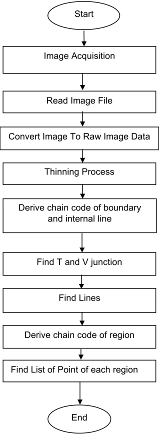
Figure 1 shows modules involved from image acquisition to acquiring a junction, line and region table. Each module is explained in the next sections.
2.0 DEFINITION
In this paper, several terms used are briefly defined. They will be used frequently in the discussion.
Chain Code
Chain Code is a list of code range from number zero to seven in clockwise direction. The codes represent direction of the next pixel connected in window 3×3 as shown in Figure 2. There are eight locations of pixels that surrounding the current pixel that is represented by row and column. For example, in the code 0, the coordinate is (row, column+1).
Raw Image
Raw image is an image file contains only data of the image without header or other information about the image. The data is extracted from other image file formats such as TIFF, PCX or JPEG.
Line drawing
Line drawing is a drawing with no shadow, range and pattern. It can be divided into two types; namely regular and irregular image. Regular line drawing is a drawing where line is drawn straight without any extra corner. Irregular line drawing is a draw-ing where a line is not drawn straight. Therefore, a line may appear as two or more connected lines.
Trihedral object
Figure 1 System Flowchart Start
Thinning Process
Derive chain code of boundary and internal line
Find Lines
Derive chain code of region
Find List of Point of each region Find T and V junction
End Read Image File
Convert Image To Raw Image Data Image Acquisition
Figure 2 Chain Code & Their Locations column-1 column column+1
row-1 5 6 7
row 4 (current
pixel) 0
shared by exactly three faces then the object is called a trihedral object. For example, a four-faced pyramid is not called trihedral object because the peak is shared by four faces.
3.0 DATA STRUCTURE INVOLVED
This section explains data structure used by the algorithm in deriving junctions, lines and regions of the irregular line drawing.
Array of Image
Array of Image is a two-dimensional array with type char. It keeps binary image that consists of two values namely ‘0’ and ‘1’. These values are obtained from threshold process of the raw data.
Table of Boundary and Internal Chain Code
The list consists of three fields namely row, column and code. Row and column repre-sent position of the pixel in the image. Code reprerepre-sents chain code of the pixel as explained in Section 2. The code field in the last record of the list is valued –1 to indicate that there is no more pixel.
For boundary list, the row and column of the last record must be adjacent to the first record because it keeps all record of pixels bounded the drawing.
Table of Region Chain Code
The list consisted of three fields namely row, column and code. The first record con-tains T-junction on boundary. The last record of the list is adjacent to the first record. The list is used to derive the list of points that bounded the region.
Table of Junction
The table consisted of four fields namely point_number, row, column, and junction_type. Point_number is an index of the table. Row and column represents coordinate of the junction. Junction type is a code that is representing the junction type. The codes are 2, 3 and 99 that representing V-junction, T-junction on boundary and T-junction on inter-nal line.
Table of Line
represents line with type arrow, plus and minus respectively. For line with type arrow, the direction is from the StartPoint to EndPoint. The symbols that representing the line type is in fact to be used in Picture Description Language and the convention follows the Huffman[10] line labeling. The line labeling is not discussed in this paper.
Table of Region
The table consisted of two fields namely Region_number and Point_list. Region_number is an index of the table. A region is bounded by a series of junctions. Point_list is a linked list used to keep the list of junction numbers that bounded the region. The junction numbers are the number found in Table of Junction.
4.0 ACQUIRING BINARY IMAGE
As shown in Figure 1, this section explains the first three modules of the processing namely image acquisition, read image file and convert image file to binary data.
There are two ways to acquire image. First, image is acquired by sketching the drawing using any image editor such as Adobe Photoshop and then the image is saved in a file as TIFF format. Second, using a sheet of paper and a pencil or pen, a drawing is sketched. Then, it is scanned and saved as TIFF image. None of the method required programming function.
Reading the TIFF is done by creating a C function. The input of the function is the TIFF image file. The output is an array consists of pixel value of the image.
In converting the image file into binary data, a C function is created. The input of the function is image array consists of the original pixel value. The output is a new image array consists of binary data of the original image. For this purpose, a threshold value 200 has been chosen.
5.0 THINNING PROCESS
Thinning can be defined heuristically as a set of successive erosions of the outermost layers of a shape, until a connected unit-width set of lines (skeleton) is obtained [9]. Thus, thinning algorithms are iterative algorithms that ‘peel off’ border pixels, i.e. pixels lying at 0 → 1 transitions in a binary image. Connectivity is an important prop-erty that must be preserved in the thinned object. Therefore, border pixels are de-tected in such a way that object connectivity is maintained. To suit the chain code algorithm, two stages are required in the thinning process.
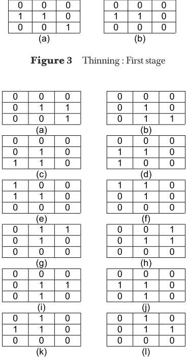
As in the first stage, the second stage of thinning process is also to ensure that the removal of current pixel will not shorten an object limb. The difference is the total pixel ‘1’ of the neighborhood pixel from 2 to 3 or 4. In other words, it also ensures that there is no excess pixel in the window 3×3.
For total pixel ‘1’ of the neighborhood is equal to 2, then there are twelve cases to be considered as shown in Figure 4.
0 0 0 0 0 0
0 1 1 0 1 0
0 0 1 0 1 1
(a) (b)
0 0 0 0 0 0
0 1 0 1 1 0
1 1 0 1 0 0
(c) (d)
1 0 0 1 1 0
1 1 0 0 1 0
0 0 0 0 0 0
(e) (f)
0 1 1 0 0 1
0 1 0 0 1 1
0 0 0 0 0 0
(g) (h)
0 0 0 0 0 0
0 1 1 1 1 0
0 1 0 0 1 0
(i) (j)
0 1 0 0 1 0
1 1 0 0 1 1
0 0 0 0 0 0
(k) (l)
Figure 4 12 cases where total pixel ‘1’ of the neighborhood is equal to 2
Figure 3 Thinning : First stage
0 0 0 0 0 0
1 1 0 1 1 0
0 0 1 0 0 0
(a) (b)
For total pixel ‘1’ of the neighborhood is equal to 4, then there are twelve cases to be considered as shown in Figure 5.
6.0 BOUNDARY AND INTERNAL LINE: CHAIN CODE PRO-CESSING METHODOLOGY
This section explains in detail how to derive boundary and internal line chain code by using Figure 6 as an example. There is only one boundary chain code and one inter-nal line chain code representing Figure 6. These chain codes are used to determine junction coordinate and junctions that connect two lines. The code of locations in Figure 6 must be referred along the discussion. Explanation is divided into two parts namely boundary searching and internal line searching. The boundary chain code must be derived first so that internal line searching will concentrate in the inner part of the drawing. This work only focused on image with one closed area consisted of more than region. In other words, this work only cater for series of chain code consists of one boundary chain code and more than internal line chain code. For the purpose of explanation, only one internal line chain code has been chosen.
Boundary Searching
Firstly, find the first pixel in the image by traverse by column and followed by row. The first pixel found will be the start of the boundary chain code. Starting from that pixel, window 3×3 of the coordinate is selected. The first pixel found in the clockwise direction (refer to Figure 2) of the window will be the next testing pixel. For example,
Figure 5 12 cases where total pixel ‘1’ of the neighborhood is equal to 4
0 1 0 0 1 0
1 1 1 0 1 1
0 0 0 0 1 0
(a) (b)
0 0 0 0 1 0
1 1 1 1 1 0
0 1 0 0 1 0
(c) (d)
1 1 0 0 0 1
0 1 1 0 1 1
0 0 0 0 1 0
(e) (f)
0 0 0 0 1 0
1 1 0 1 1 0
0 1 1 1 0 0
(g) (h)
0 1 0 0 0 0
0 1 1 0 1 1
0 0 1 1 1 0
(i) (j)
1 0 0 0 1 1
1 1 0 1 1 0
0 1 0 0 0 0
at coordinate (1,3) Figure 7, location code 0 should be the next test pixel and not location code 3. The selection is determined by selecting the start location of traverse.
Figure 6 Example of Binary Image 0 1 2 3 4 5 6 7 8 0
1 1 1
2 1 1
3 1 1 1
4 1 1 1
5 1 1 1 1
6 1 1 1 1 1
7 1 1
8 1 1 1 1 1 9
0 0 0
0 1 1
1 0 0
Figure 7 First Pixel at Coordinate (1,3)
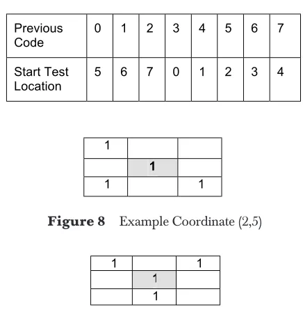
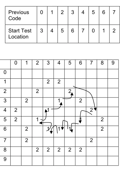
To determine the start test location in the window, the previous connected pixel need to be checked. For the first pixel, it is assumed that the previous pixel is from location 0 or otherwise the start test location is based on the previous location code. Table 1 shows the start test location based on the previous location code.
Figure 8 shows window 3×3 of coordinate (2,5) of image in Figure 6. The previous connected pixel is from coordinate (1,4) and the previous location code is 1. There are two pixels connected to the current pixel namely at location 1 and 3. Based on Table 1, the start of search location for previous location code 1 is at location 6 in clockwise direction. There is no pixel at location 6, 7 and 0. The first pixel ‘1’ is found at location 1. Therefore, the connected pixel is at coordinate (3,6) and the previous location code is 1.
Previous
Code 0 1 2 3 4 5 6 7
Start Test
Location 5 6 7 0 1 2 3 4
Table 1 Start Test Location (clockwise direction)
1
1
1 1
Figure 8 Example Coordinate (2,5)
Figure 9 Example Coordinate (6,1): Row 6 and Column 1
1 1
1
1
Therefore, current pixel changed to coordinate (5,0) and the location code changed from 6 to 5.
Deriving the boundary chain code stop when the current pixel is the first pixel found in the array. Figure 10 shows pixel after the boundary chain code derived. The pixel with number 2 indicated that the pixels are already traversed as a boundary pixel.
Internal Line
Using the array of image shown in Figure 10, the searching of internal line chain code is proceeded. As the process continued, the values of all the traversed pixel will be changed to ‘2’. The conversion is to indicate that the pixel is already belonging to a boundary. There is a difference between internal line chain code compared to bound-ary line processing algorithm in term of how the traversal is terminated. The traversal of boundary line is terminated when pixel location is back to the first pixel found while for internal line, the traversal is terminated when the first pixel valued 2 found. The similarity between these algorithm is that the first search pixel of internal line and boundary line is the first pixel that is not traversed yet or the pixel value is equal to 1. Therefore, there may be more than one internal line chain code.
next connected pixel is at location 3 and the coordinate is (4,3). Figure 10 Array of Image after boundary chain code derived
0 1 2 3 4 5 6 7 8 9 0
1 2 2
2 2 2
3 2 1 2
4 2 1 2
5 2 1 1 2
6 2 1 1 1 2
7 2 2
8 2 2 2 2 2
9
Figure 11 Coordinate (3, 4)(2: indicate boundary pixel) 2
1
1
Searching result of the boundary and internal line chain code for Figure 6 is as shown below where –1 indicate last pixel of the list.
Boundary:
Start at (1,3): 0111123344445656777-1
Internal Line:
Start at (3,4):331007-1
6.1 Junction Searching
This section explains algorithm to find junction given a boundary chain code and internal line chain codes. Line intersection is applied to find the junction. The discus-sion is divided into two parts namely T-junction and V-junction. T-junctions are de-rived first because they will be used in finding the V-junctions.
T-Junction
There are two types of T-junction, which are located on the boundary line and which are located on the internal line. The T-junction on boundary is derived first then fol-lowed by T-junction on internal line.
For every coordinate in the boundary chain code, they are compared to the first and last record of all the internal line chain code. If current boundary coordinate is adja-cent to those records, then the boundary coordinate will be assigned as T-junction with type 3.
T-junction on internal line is derived by comparing all coordinates in the current internal line chain code. These values are compared to the first and last records of the rest of internal line chain code. If adjacent coordinate is found, then the T-junction with type 99 will be assigned to the coordinate. The comparison is done to all internal lines. Table of Junction will be created when the process is completed.
V-Junction
The boundary and internal line chain code is still referred in deriving V-junction. For every chain code, the coordinates of consecutive T-junctions on the chain code is identified. Codes between these coordinates will be copied into a temporary chain
2
1
2 1
code. For boundary chain code, since the first pixel is not necessarily T-junction, the last record of the list will be linked to the first record of the list. The algorithm ex-plained below is based on the temporary chain code consists of nine codes between two coordinates of T-junctions.
More than one V-junction can be found between coordinates of T-junctions. If there is more than nine codes/pixels between the T-junctions, this algorithm will be repeated until no more pixel to be traversed. If less than nine codes exist between coordinates of T-junctions, it is assumed that no V-junctions between the coordinates of T-junctions. For example, if there are m codes between T-junctions, it means the process to find V-junction is repeated m-8 times.
For each temporary chain code created, nine coordinates of row and column founded in the chain code is segmented and tested. They are extracted by their appearance in the list and the row and column values are kept in an array called ArrayOfRow and ArrayOfColumn respectively. The coordinate values of row and column are manipu-lated as follows.
1. Using Equation 1, calculate the sum of difference of rows.
1 2
= −
DiffRow R R (1)
where
3
0 7
4
1 [ ( 1) ( )]
2 [ ( 1) ( )] =
=
= + −
= + −
∑
∑
n
n
R R n R n
R R n R n
R is array of row
n is number of pixel tested
2. Using Equation 2, calculate the sum of difference of columns.
1 2
= −
DiffCol C C (2)
where
3
0 7
4
1 [ ( 1) ( )]
2 [ ( 1) ( )] =
=
= + −
= + −
∑
∑
n
n
C C n C n
R is array of row
n is number of pixel tested
3. Using Equation 3, calculate the total of the differences.
Total = |DiffRow| + |DiffCol| (3)
4. If (Total > 3) then
the value in array row and column of index number 4 is a junction.
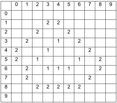
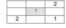
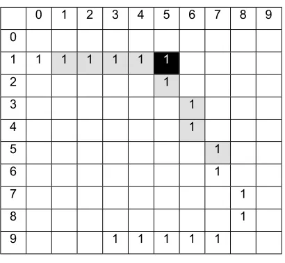
Figure 13 shows an example of image consisting of two V-junctions at coordinate (1,5) and (8,8). It is assumed that the coordinate (1,0) and (9,3) are T-junction. Since there are 18 codes between the coordinates, the process has to be repeated ten (18-8) times. The process will create ten segments of nine coordinates of row and column. For the first segment, the start, last and testing coordinates are at coordinate (1,0), (4,6) and (1,4) respectively. For the last or the tenth segment, the start, last and testing coordinates are at coordinate (5,7), (9,3), and (9,7) respectively.
Figure 13 V-junction at coordinate (1,5) 0 1 2 3 4 5 6 7 8 9 0
1 1 1 1 1 1 1
2 1
3 1
4 1
5 1
6 1
7 1
8 1
9 1 1 1 1 1
Table 2 Content of Array Row and Column No Row Col
0 1 1
1 1 2
2 1 3
3 1 4
4 1 5 Í Testing Coordinate
5 2 5
6 3 6
7 4 6
8 5 7
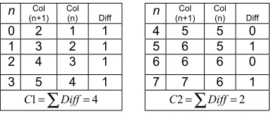
The total of the row and column differences is calculated as shown in Table 5.
n Row
(n+1) Row (n) Diff n (n+1)Row Row (n) Diff
0 1 1 0 4 2 1 1 1 1 1 0 5 3 2 1 2 1 1 0 6 4 3 1 3 1 1 0 7 5 4 1
0 1=∑Diff=
R R2=∑Diff=4
Table 3 Sum of Difference of Rows
n Col
(n+1) Col (n) Diff n (n+1)Col Col (n) Diff
0 2 1 1 4 5 5 0 1 3 2 1 5 6 5 1 2 4 3 1 6 6 6 0 3 5 4 1 7 7 6 1
4 1=∑Diff=
C C2=∑Diff=2
Table 4 Sum of Difference of Columns
Using the values in Table 2, the sum of the difference of rows is calculated as shown in Table 3.
Using the values in Table 2, the sum of the difference of columns is calculated as shown in Table 4.
DiffRow = R1 R2 = 0 4 = 4
DiffCol = C1 C2 = 4 2 = 2
Total = |DiffRow| + |DiffCol| = 4 + 2 = 6
Since the total of difference is greater than 3, then row 1 and column 5 are assigned as a V-junction.
Since the image is irregular, there is a possibility of two consecutive V-junction derived from the calculation. Verification of existence of any V-junction must be done before inserting the row and column into table of junction. For every V-junction, if the current coordinate is found adjacent to any junction in the table, then the coordinate will be replaced with the new coordinate found with type 2.
The algorithm can also be applied to a single series of chain code with the assump-tion that the first and the last pixel is a T-juncassump-tion.
6.2 Line Searching
Lines are derived from boundary and internal line. They are also associated with the junctions created before. The discussion is divided into the search of the junctions founded in the boundary and internal line.
For chain code boundary, coordinate for each record in the chain is compared to the row and column in Table of Junction. The first coordinate that matches the coordi-nate in junction table is assigned as start point of the current line. After the first point is founded, the next point in the list is searched. The next point found will be the end of the current line and start of next line. The chain code is continuously traversed and every point founded will be assigned as end and start point of the current line and next line respectively. When the list terminator founded, and then the first point found in the list is assigned as end of the current line and this indicate the end of line search of boundary chain code.
Next step is to find line of internal line. There are two differences between line searching on boundary and internal line chain code. First, coordinate of junction in boundary line can be found exactly as in the junction table while the coordinate of junction in internal line may be adjacent to the coordinate in the table. Therefore, to find the junction in the internal line, checking must be done to find coordinate that is adjacent to coordinate in the table. Secondly, the last coordinate in internal line chain code is the end of current line.
For each internal line, start coordinate and end coordinate of the list is a start and end of first and last line in the list. The junction found between these junctions would be end and start point of the current line and next line in the list respectively. The lines found are kept in table of line.
6.3 Region: The Chain Code Processing Algorithm
First step is to determine number of regions found in the image based on the num-ber of T-junction on boundary. Next, for all T-junction along the boundary, the region chain code is derived.
For every T-junction, the record of chain code between the T-junction and the next consecutive T-junction is copied into region code. Starting from the next T-junction, the connected pixel in the window 3×3 is determined using the previous location code of the current pixel. Starting from the start location, the window is traversed in anti-clockwise direction.
The discussion is referring to binary image in Figure 10. Figure 14 shows directions of the code produced for the first region. Starting from the first T-junction on bound-ary located at coordinate (2,5), the records are copied into region code until next T-junction at coordinate (4,7) is found. At coordinate (4,7), the previous code is 1. Using Table 6, the start test location is 4 and followed by 3, 2, 1, 0, 7, 6 and 5. The testing gives location 3 as the next connected pixel. The process is continued until the search pixel return to the start pixel i.e. at (2,5) and created a first region chain code of the image.
Figure 14 Direction of chain code for the first region 0 1 2 3 4 5 6 7 8 9 0
1 2 2
2 2 2
3 2 1 2
4 2 1 2
5 2 1 1 2
6 2 1 1 1 2
7 2 2
8 2 2 2 2 2
9
Previous
Code 0 1 2 3 4 5 6 7
Start Test
Location 3 4 5 6 7 0 1 2
Figure 15 shows directions of the code produced for the second region. The current T-junction is at coordinate (4,7). From the point, the next T-junction on the boundary is at coordinate (6,1). From the coordinate (6,1) and using Table 6 to determine the next pixel, the second region is found when the traversal return to coordinate (4,7).
Figure 16 shows directions of the code produced for the third region. The current T-junction is at coordinate (6,1). From the point, the next T-T-junction on the boundary is at coordinate (2,5). From the coordinate (2,5) and using Table 6 to determine the next pixel, the third region is found when the traversal return to coordinate (6,1). The total number of region of Figure 10 is three.
0 1 2 3 4 5 6 7 8 9 0
1 2 2
2 2 2
3 2 1 2
4 2 1 2
5 2 1 1 2
6 2 1 1 1 2
7 2 2
8 2 2 2 2 2
9
Figure 15 Direction of chain code for the second region
Figure 16 Direction of chain code for the third region
0 1 2 3 4 5 6 7 8 9 0
Using the region chain code, a region table is created by comparing the coordinate in the record that match or adjacent to the coordinate in table of junction. Once the junction is found, the list of point bounded the region is created for each region.
7.0 EXPERIMENTAL RESULTS
The chain code algorithm is tested using four test data namely cube, stair, L-block and n -block with image size is 100×100, 50×50, 100×100 and 100×100 respectively. The algo-rithm is tested and the output of each test data is shown in this section. The algoalgo-rithm written cannot accept input where the line is uncompleted such as shown in Figure 20. We divide discussion into four parts namely the cube, stair, L-block and n-block.
Cube 100 × 100
Figure 17 shows the input TIFF file image. Table 7 shows the list of junction and lines extracted from the drawing. Table 8 shows the list of region and its list of point bounded the region. Table 9 and 10 shows the chain code of boundary and internal line and region.
Table 7 Junction & Line Table of Cube Figure 17
JUNCTION TABLE
Row Col PntNo PntType === === ===== =======
3 8 7 0 0 3
8 4 4 1 1 3
3 4 1 5 2 3
5 5 4 0 3 9 9
6 4 7 1 4 2
7 0 1 5 5 2
1 6 4 7 6 2
LINE TABLE
Line Line S t E n d N o Type = = = = = = = ====
7 0 0 1
0 4 1 1
4 1 2 1
1 6 3 1
6 2 4 1
2 7 5 1
2 3 6 9 9
3 0 7 9 9
3 1 8 9 9
Table 8 Region Table of Cube Figure 17
REGION TABLE
List of Point in Region 0: 0 4 1 3 List of Point in Region 1: 1 6 2 3 List of Point in Region 2: 2 7 0 3
Stair 50 × 50
Figure 18 shows the input TIFF file image. Table 11 shows the list of junction and lines extracted from the drawing. Table 12 shows the list of region and its list of point bounded the regions. Table 13 and 14 shows the chain code of boundary and internal line and region.
Table 9 Chain Code of Boundary and Internal Line of Cube Figure 17
CHAIN CODE: BOUNDARY AND INTERNAL LINE
Start From (16,45)
–1001011012111111101011111112211222222222221222222222 233343434443343333334333343333434334545555554555445454 554556665666666666666666666666666665666777770700700770 0077707707707770
Start From (35,16)
–10112101101111111110111101700777070700070707007770770707
Start From (56,40) –1222222222222222222222222222
Table 10 Chain Code of Region of Cube Figure 17
CHAIN CODE: REGION
Start From (38,70)
–111222222222221222222222233343434443343333334333343 333434566666666666666666666666666667007770707000707070 07770770707
Start From (84,41)
–133454555555455544545455455666566666666666666666666 666666566677101121011011111111101111012222222222222222 222222222222
Start From (34,15) –177707007007700077707707707770–1001
011012111111101011111112223434334333443434344434343334435455554555 555555455456554
Table 12 Region Table of Stair Figure 18
REGION TABLE
List of Point in Region 0: 0 12 1 11 10 9 8 7 List of Point in Region 1: 1 13 2 11
List of Point in Region 2: 2 3 10 11 List of Point in Region 3: 3 4 9 10 List of Point in Region 4: 4 5 8 9 List of Point in Region 5: 5 6 7 8 List of Point in Region 6: 6 14 0 7
Table 11 Junction & Line Table of Stair Figure 18
JUNCTIONTABLE
R o w C o l PntNo PntType = = = ==== ===== ======
9 3 9 0 3
4 4 1 7 1 3
2 8 5 2 3
2 6 1 2 3 3
1 7 1 5 4 3
1 4 2 0 5 3
7 2 1 6 3
1 5 3 3 7 9 9
1 9 3 1 8 9 9
2 4 2 4 9 9 9
3 2 2 3 1 0 9 9
3 6 1 7 1 1 9 9
3 3 4 0 1 2 2
3 4 4 1 3 2
2 2 7 1 4 2
LINE TABLE
From T o LineNo LineType ==== = = ====== ========
1 4 0 0 1
0 1 2 1 1
1 2 1 2 1
1 1 3 3 1
1 3 2 4 1
2 3 5 1
3 4 6 1
4 5 7 1
5 6 8 1
6 1 4 9 1
6 7 1 0 9 9
7 0 1 1 9 9
5 8 1 2 9 9
8 7 1 3 9 9
4 9 1 4 9 9
9 8 1 5 9 9
9 1 0 1 6 9 9
1 0 1 1 1 7 9 9
1 1 1 1 8 9 9
3 1 0 1 9 9 9
2 1 1 2 0 9 9
Table 13 Chain Code of Boundary and Internal Line of Stair Figure 18
BOUNDARY AND INTERNAL LINE
Start From (1,26)
–1110101011001111222222222222222222222333433443443443 4334334354445555555555666667700007076666
6667070707666666767777
Start From (7,22) –11110101011177777
Start From (15,21) –10101001010767
Start From (18,16) –111101011000070776
Start From (25,24) –1222222323434432222222
Start From (26,13) –1111010101
L-block 100 × 100
Figure 19 shows the input TIFF file image. Table 15 shows the list of junction and lines extracted from the drawing. Table 16 shows the list of region and its list of point bounded the region. Table 17 and 18 shows the chain code of boundary and internal line and region.
Table 14 Chain Code of Region of Stair Figure 18
REGION
Start From (9,39
–111222222222222222222222333433443443443433433435 66666666700707676666667000707765767677777
Start From (44,17) –144455555555556666671101101010112222222
Start From (28,5) –170000700111010101134344355454545545
Start From (26,12) –17666666670111101011222222234545454555
Start From (17,15) –17070710101001010123343444455454555
Start From (14,20) –1666666701110101011123234545445454
Start From (7,21) –167777–1110101011001133333355545454555
Figure 19 L-block size 100 ×100
Table 15 Junction & Line Table of L-block Figure 19
JUNCTIONTABLE
R o w C o l PntNo PntType = = = ==== ===== ======
4 7 8 4 0 3
9 1 7 0 1 3
7 6 4 7 2 3
8 4 3 0 3 3
2 8 1 2 4 3
5 5 3 1 5 9 9
4 8 4 9 6 9 9
6 0 6 9 7 9 9
9 1 6 5 8 2
8 4 2 6 9 2
2 2 1 3 1 0 2
7 4 0 1 1 2 2
LINE TABLE
From T o LineNo LineType ==== = = ====== ========
1 1 0 0 1
0 1 1 1
1 8 2 1
8 2 3 1
2 3 4 1
3 9 5 1
9 4 6 1
4 1 0 7 1
1 0 1 1 8 1
4 5 9 9 9
5 6 1 0 9 9
6 7 1 1 9 9
7 0 1 2 9 9
6 2 1 3 9 9
5 3 1 4 9 9
Table 16 Region Table of L-block Figure 19
REGION TABLE
List of Point in Region 0: 0 1 7 List of Point in Region 1: 1 8 2 6 7 List of Point in Region 2: 2 3 5 6 List of Point in Region 3: 3 9 4 5
List of Point in Region 4: 4 10 11 0 7 6 5
Table 17 Chain Code of Boundary and Internal Line of L-block Figure 19
CHAIN CODE : BOUNDARY AND INTERNAL LINE
Start From (7,38
-100111101010110101101101110111011111111221111112122 1112222222221222222222222223233332333332333334443454 5555455455555555453434343433334344534455556555656565 5665566555656665666666666666666666666666777566677000 077077707777707707700
Start From (28,13)
–11121121212121211211211121110070707077077700010000101 011011111110107077777777777
Start From (49,48) –122222222222222232222222222
Start From (56,31) –1322222222222222222222222222
Start From (61,69) –122222222222222222222222222222
Table 18 Chain Code of Region of L-block Figure 19
CHAIN CODE : REGION
Start From (47,84)
–11122222222212222222222222232333323333323333344566666 66666666666666666666666677077777777777
Start From (91,70)
–1434545555455455555555456666666666676666666666666667 00001010110111111101222222222222222222222222222222
Start From (76,47)
–1343434343333434456666666666666666666666666667707070 707707770001322222222222222232222222222
Start From (84,30)
–1344555565556565655665566555656665666666666666666666 666666777011211212121212112112111211123222222222222222 22222222222
Start From (28,12)
-1566677000077077707777707707700-100111101010110101101 101110111011111111221111112122133333333333343454555555 545545454444544433343343434344555655565565565656565655 6 5 5
n-block 100×100
Figure 20 shows irregular line drawing with a uncompleted line. This type of drawing is not considered in this work. Future works can be considered to extract regions of the drawing.
Figure 20 n-Block size 100 ×100 (unacceptable input)
Uncompleted line
8.0 CONCLUSIONS AND FUTURE WORKS
This section is divided into two parts namely to conclude and to propose future work of the study. The first section discusses four issues that have been improved from previous research namely input technique of line drawing interpreter, thinning algo-rithm, chain code algoalgo-rithm, and V-junction detection. The second section suggests future works to improve the current results. There are four suggestions proposed in this paper namely wide range of input object, optimizing the threshold value, optimiz-ing the parameter of code length, and improvoptimiz-ing the thinnoptimiz-ing algorithm.
8.1 Conclusions
One of the objective of this work is to propose new method to derive a geometric entity of a line drawing given a chain code series as the input. The three objects used in the experiment have yielded junctions, lines and regions which are representing the geometry of the drawing. The output can be used as input of the system proposed by Grimstead[3]. The output also can be used in line labeling process of Huffman[10] and Mackworth[11] by applying the line_type field in the Table of Line. The method also simplify the process of extracting basic entity of a line drawing without using any sketch interpreter.
For thinning algorithm, besides detecting total pixel ‘1’ of the neighbourhood is 1, this work has extended works by Pitas[2] and Sulong[6] in terms of detecting that the total pixel ‘1’ of the neighborhood is 2 or 3. In addition, this algorithm has maintained the basic shape and size of the line drawing.
object. Based on the chain code proposed by Pitas[9], the effect of direction in the traversal of codes has been studied and used to identify region of a closed area.
In finding V-junction, the method proposed here have utilized the chain codes derived. This work has also chosen parameter nine based on the work proposed by Rabu[13]. By combining the chain code derived and through simple calculations, V-junctions can be detected. Experiment results show that nine is suitable for image size 50×100 and 100×100. This conclusion is supported by Rabu[13].
8.2 Future Works
There are four inputs tested on the system. The input consists of unconnected line has not been tested in the algorithm. The algorithm proposed can be modified so that is can accept input of the unconnected line. In fact, if there is unconnected line, the algorithm should be able to suggest and connect the line to the potential junction as proposed by Grimstead[3].
The number of threshold chosen is 200. The number is chosen with the basis that it is suitable enough to convert grey level values range from 0 to 255 to binary values 0 and 1.
The parameter code length chosen in this study in determine the V-junction is actually can still be optimized. Extensive research can be done to formulate how the algorithm can automatically determine the optimum parameter value based on the image size and the length of the codes. Therefore, instead of value nine, the number should be assigned by the system.
In the thinning algorithm, since the traversal started from left to right, therefore the eliminating of the pixel is left-oriented. As a result, the thinned image is not really representing actual form of the drawing. It is suggested that instead of 3×3 window, bigger window can be considered so that more surrounding pixels will be taken in consideration in thinning process. Eventhough this study have used thinning process by Sulong[12] as the basis, the work also did not consider about the effect of left-orientation of the thinning process.
To summarize, this paper has succeeded to propose a new type of input of the line drawing interpreter, improving thinning and chain code algorithm and propose new method to find V-junction of irregular line drawing. Further, by testing on wide range of objects such as unconnected line and variety of image size, the existing methodol-ogy can be improved and be an alternative to the existing line drawing interpreter.
ACKNOWLEDGEMENT
REFERENCES
[1] Freeman, H. 1974. Computer Processing of Line-Drawing Images. Computing Surveys. 6(1).
[2] Jenkins, D.L. 1992. “The Automatic Interpretation of Two-Dimensional Freehand Sketches”, PhD Thesis, Department of Computing Mathematics, University of Wales, Cardiff, U.K.
[3] Grimstead, I.J. 1997. “Interactive Sketch Input of Boundary Representation Solid Models”, PhD Thesis, Department of Computing Mathematics, University of Wales, Cardiff, U.K.
[4] Varley, P.A.C. and R.R. Martin. 2000. “ A system for Constructing Boundary Representation Solid Models from a Two-Dimensional Sketch-Geometric Finishing”, 1st Korea-UK Joint Workshop on Geometric Mod-eling and Computer Graphics.
[5] Varley, P.A.C. and R.R. Martin. 2000. “A System for Constructing Boundary Representation Solid Models from a Two-Dimensional Sketch”, Proceedings of Geometric Modeling and Processing 2000: Theory and Applications. 13-32.
[6] Liu, J.Z., W.K. Cham, Q.R. Chen and H.T. Tsui. 2001. “3D surface reconstruction from single 2D line drawings and its application to advertising on the internet”, Proceedings of 2001 International Symposium on Intelligent Multimedia, Video and Speech Processing. 453-456.
[7] Bribiesca, E. 2000. “A chain code for representing 3d curves”, Pattern Recognition. (33):755-765. [8] Bribiesca, E. 1999. “A new chain code”, Pattern Recognition. (32):235-251.
[9] Pitas, I. 1995. Digital Image Processing Algorithm. University Press Cambridge, Prentice Hall.
[10] Huffman, D.A. 1971. Impossible Objects as Nonsense Sentences, pages 295-323. Machine Intelligence 6. New York: American Elseiver.
[11] Mackworth, A.K. 1973. Interpreting Pictures of Polyhedral Scenes. Artificial Intelligence. 4:121-137. [12] Sulong, S.M. 1999. Pengecaman Cap Jari: Penipisan Imej Menggunakan Algoritma Penipisan Berselari. BSc
Thesis Universiti Technologi Malaysia.
01234567890123456789012345678901234567890123456789 0 00000000000000000000000000000000000000000000000000 1 00000000000000000000000001100000000000000000000000 2 00000000000000000000000011011000000000000000000000 3 00000000000000000000000110001110000000000000000000 4 00000000000000000000001100000011100000000000000000 5 00000000000000000000011000000000110000000000000000 6 00000000000000000000010000000000001100000000000000 7 00000000000000000000111000000000000111100000000000 8 00000000000000000000110100000000000000110000000000 9 00000000000000000000100011000000000000011100000000 10 00000000000000000000100001110000000000111100000000 11 00000000000000000000100000011100000001100100000000 12 00000000000000000000100000000111000011000100000000 13 00000000000000000000100000000001101100000100000000 14 00000000000000000000100000000000111000000100000000 15 00000000000000000111111000000000010000000100000000 16 00000000000000011100000111000000110000000100000000 17 00000000000001110000000001111000100000000100000000 18 00000000000001011000000000001110100000000100000000 19 00000000000001001110000000000011100000000100000000 20 00000000000001000011000000000001100000000100000000 21 00000000000001000001110000000000100000000100000000 22 00000000000001000000011100000011100000000100000000 23 00000000000001000000000110001110000000000100000000 24 00000000000001000000000011111000000000000100000000 25 00000000000001000000000010000000000000000100000000 26 00000000000111000000000010000000000000000100000000 27 00000111111000100000000010000000000000000100000000 28 00001100000000011000000010000000000000000100000000 29 00001011000000001110000010000000000000000100000000 30 00001001110000000011100010000000000000000100000000 31 00001000011000000000111010000000000000001100000000 32 00001000001110000000001110000000000000011100000000 33 00001000000011100000000110000000000000001100000000 34 00001000000000111000111100000000000000110000000000 35 00001100000000001111100000000000000011100000000000 36 00000110000000000100000000000000000110000000000000 37 00000011000000000100000000000000111100000000000000 38 00000000110000000100000000000111100000000000000000 39 00000000010000000100000000111100000000000000000000 40 00000000001000000100000011100000000000000000000000 41 00000000001100000100000110000000000000000000000000 42 00000000000110000100011100000000000000000000000000 43 00000000000011100100110000000000000000000000000000 44 00000000000000111111100000000000000000000000000000 45 00000000000000001111000000000000000000000000000000 46 00000000000000000000000000000000000000000000000000 47 00000000000000000000000000000000000000000000000000 48 00000000000000000000000000000000000000000000000000 49 00000000000000000000000000000000000000000000000000 01234567890123456789012345678901234567890123456789 Appendix A
Figure 21 RawFile From TIFF Image Figure 22 After Thin Process
Figure 23 Boundary, Internal Line and Region List BOUNDARY AND INTERNAL LIST List of Direction 0: Row Col Code 1 26 -1 2 27 1 3 28 1 3 29 0 4 30 1 4 31 0 5 32 1 5 33 0 6 34 1 7 35 1 7 36 0 7 37 0 8 38 1 9 39 1 10 40 1 11 41 1 12 41 2 13 41 2 14 41 2 15 41 2 16 41 2 17 41 2 18 41 2 19 41 2 20 41 2 21 41 2 22 41 2 23 41 2 24 41 2 25 41 2 26 41 2 27 41 2 28 41 2 29 41 2 30 41 2 31 41 2 32 41 2 33 40 3 34 39 3 35 38 3 35 37 4 36 36 3 37 35 3 37 34 4 37 33 4 38 32 3 38 31 4 38 30 4 39 29 3 39 28 4 39 27 4 40 26 3 40 25 4 41 24 3 42 23 3 42 22 4 43 21 3 44 20 3 44 19 4 45 18 3 44 17 5 44 16 4 44 15 4 44 14 4
Appendix B
43 13 5 42 12 5 41 11 5 40 10 5 39 9 5 38 8 5 37 7 5 36 6 5 35 5 5 34 4 5 33 4 6 32 4 6 31 4 6 30 4 6 29 4 6 28 5 7 27 6 7 27 7 0 27 8 0 27 9 0 27 10 0 26 11 7 26 12 0 25 13 7 24 13 6 23 13 6 22 13 6 21 13 6 20 13 6 19 13 6 18 13 6 17 14 7 17 15 0 16 16 7 16 17 0 15 18 7 15 19 0 14 20 7 13 20 6 12 20 6 11 20 6 10 20 6 9 20 6 8 20 6 7 21 7 6 21 6 5 22 7 4 23 7 3 24 7 2 25 7
List of Direction 1: Row Col Code 7 22 -1 8 23 1 9 24 1 10 25 1 10 26 0 11 27 1 11 28 0 12 29 1 12 30 0 13 31 1 14 32 1 15 33 1 14 34 7 13 35 7 12 36 7 11 37 7 10 38 7
List of Direction 2: Row Col Code 15 21 -1 15 22 0 16 23 1 16 24 0 17 25 1 17 26 0 17 27 0 18 28 1 18 29 0 19 30 1 19 31 0 18 32 7 17 32 6 16 33 7
List of Direction 3: Row Col Code 18 16 -1 19 17 1 20 18 1 21 19 1 21 20 0 22 21 1 22 22 0 23 23 1 24 24 1 24 25 0 24 26 0 24 27 0 24 28 0 23 29 7 23 30 0 22 31 7 21 32 7 20 32 6
List of Direction 4: Row Col Code 25 24 -1 26 24 2 27 24 2 28 24 2 29 24 2 30 24 2 31 24 2 32 23 3 33 23 2 34 22 3 34 21 4 35 20 3 35 19 4 35 18 4 36 17 3 37 17 2 38 17 2 39 17 2 40 17 2 41 17 2 42 17 2 43 17 2
List of Direction 5: Row Col Code 26 13 -1 27 14 1 28 15 1
29 16 1 29 17 0 30 18 1 30 19 0 31 20 1 31 21 0 32 22 1
List of Direction 6: Row Col Code 29 6 -1 30 7 1 30 8 0 31 9 1 32 10 1 32 11 0 33 12 1 33 13 0 34 14 1 34 15 0 35 16 1
REGION LIST
Region No 0 Row Col Code 9 39 -1 10 40 1 11 41 1 12 41 2 13 41 2 14 41 2 15 41 2 16 41 2 17 41 2 18 41 2 19 41 2 20 41 2 21 41 2 22 41 2 23 41 2 24 41 2 25 41 2 26 41 2 27 41 2 28 41 2 29 41 2 30 41 2 31 41 2 32 41 2 33 40 3 34 39 3 35 38 3 35 37 4 36 36 3 37 35 3 37 34 4 37 33 4 38 32 3 38 31 4 38 30 4 39 29 3 39 28 4 39 27 4 40 26 3 40 25 4 41 24 3 42 23 3 42 22 4
43 21 3 44 20 3 44 19 4 45 18 3 44 17 5 43 17 6 42 17 6 41 17 6 40 17 6 39 17 6 38 17 6 37 17 6 36 17 6 35 18 7 35 19 0 35 20 0 34 21 7 34 22 0 33 23 7 32 23 6 31 24 7 30 24 6 29 24 6 28 24 6 27 24 6 26 24 6 25 24 6 24 25 7 24 26 0 24 27 0 24 28 0 23 29 7 23 30 0 22 31 7 21 32 7 20 32 6 19 31 5 18 32 7 17 32 6 16 33 7 15 33 6 14 34 7 13 35 7 12 36 7 11 37 7 10 38 7
Region No 1 Row Col Code 44 17 -1 44 16 4 44 15 4 44 14 4 43 13 5 42 12 5 41 11 5 40 10 5 39 9 5 38 8 5 37 7 5 36 6 5 35 5 5 34 4 5 33 4 6 32 4 6 31 4 6 30 4 6 29 4 6 28 5 7 29 6 1 30 7 1 30 8 0
31 9 1 32 10 1 32 11 0 33 12 1 33 13 0 34 14 1 34 15 0 35 16 1 36 17 1 37 17 2 38 17 2 39 17 2 40 17 2 41 17 2 42 17 2 43 17 2
Region No 2 Row Col Code 28 5 -1 27 6 7 27 7 0 27 8 0 27 9 0 27 10 0 26 11 7 26 12 0 26 13 0 27 14 1 28 15 1 29 16 1 29 17 0 30 18 1 30 19 0 31 20 1 31 21 0 32 22 1 33 23 1 34 22 3 34 21 4 35 20 3 35 19 4 35 18 4 36 17 3 35 16 5 34 15 5 34 14 4 33 13 5 33 12 4 32 11 5 32 10 4 31 9 5 30 8 5 30 7 4 29 6 5
Region No 3 Row Col Code 26 12 -1 25 13 7 24 13 6 23 13 6 22 13 6 21 13 6 20 13 6 19 13 6 18 13 6 17 14 7 17 15 0 18 16 1 19 17 1 20 18 1
21 19 1 21 20 0 22 21 1 22 22 0 23 23 1 24 24 1 25 24 2 26 24 2 27 24 2 28 24 2 29 24 2 30 24 2 31 24 2 32 23 3 32 22 4 31 21 5 31 20 4 30 19 5 30 18 4 29 17 5 29 16 4 28 15 5 27 14 5 26 13 5
Region No 4 Row Col Code 17 15 -1 16 16 7 16 17 0 15 18 7 15 19 0 14 20 7 15 21 1 15 22 0 16 23 1 16 24 0 17 25 1 17 26 0 17 27 0 18 28 1 18 29 0 19 30 1 19 31 0 20 32 1 21 32 2 22 31 3 23 30 3 23 29 4 24 28 3 24 27 4 24 26 4 24 25 4 24 24 4 23 23 5 22 22 5 22 21 4 21 20 5 21 19 4 20 18 5 19 17 5 18 16 5
Region No 5 Row Col Code 14 20 -1 13 20 6 12 20 6 11 20 6 10 20 6 9 20 6 8 20 6
7 21 7 7 22 0 8 23 1 9 24 1 10 25 1 10 26 0 11 27 1 11 28 0 12 29 1 12 30 0 13 31 1 14 32 1 15 33 1 16 33 2 17 32 3 18 32 2 19 31 3 19 30 4 18 29 5 18 28 4 17 27 5 17 26 4 17 25 4 16 24 5 16 23 4 15 22 5 15 21 4