61:1 (2013) 7–12 | www.jurnalteknologi.utm.my | eISSN 2180–3722 | ISSN 0127–9696
Full paper
Jurnal
Teknologi
Validation of Hierarchical Gene Clusters Using Repeated Measurements
Lim Fong Teea, Mohd Saberi Mohamada*, Safaai Derisa, Ahmad ‘Athif Mohd Faudzib, Muhammad Shafie Abd Latiffc, Roselina Sallehuddind
a
Artificial Intelligence and Bioinformatics Research Group, Faculty of Computing, Universiti Teknologi Malaysia, 81310 Skudai, Johor, Malaysia
bCentre for Artificial Intelligence and Robotics, Universiti Teknologi Malaysia, Jalan Semarak, 54100 Kuala Lumpur, Malaysia cPervasive Computing Research Group, Faculty of Computing, Universiti Teknologi Malaysia, 81310 Skudai, Johor, Malaysia d
Soft Computing Research Group, Faculty of Computing, Universiti Teknologi Malaysia, 81310 Skudai, Johor, Malaysia
*Corresponding author: [email protected]
Article history
Received :16 November 2011 Received in revised form : 15 December 2013
Accepted :12 February 2013
Graphical abstract
Abstract
Hierarchical clustering is an unsupervised technique, which is a common approach to study protein and gene expression data. In clustering, the patterns of expression of different genes are grouped into distinct clusters, in which the genes in the same cluster are assumed potential to be functionally related or to be influenced by a common upstream factor. Although the use of clustering methods has rapidly become one of the standard computational approaches in the literature of microarray gene expression data analysis, the uncertainty in the results obtained is still bothersome. Experimental repetitions are generally performed to overcome the drawbacks of biological variability and technical variability. In this study, the author proposes repeated measurement to evaluate the stability of gene clusters. This paper aims to prove that the stability from the gene clusters, incorporated with repeated measurement, can be used for further analysis.
Keywords:Hierachical clustering; gene clusters; repeated measurement;bootstrap procedure; stability
Abstrak
Pengklusteran hirarki adalah kaedah yang umum untuk mempelajari protein dan pengexpresan gen. Ia digunakan untuk mencari kumpulan gen atau protein. Dalam pengklusteran, pola-pola ekspressi gen yang berbeza akan dikelompokkan dalam kumpulan yang berbeza, di mana gen dalam kluster yang sama dianggap mempunyai potensi atau fungsi yang sama dan akan dipengaruhi oleh faktor yang sama. Walaupun penggunaan kaedah pengklusteran telah menjadi salah satu pendekatan pengkomputeran standard dalam kesusasteraan analisis data mikroarray pengekpresan gen, ketidaktentuan dalam keputusan yang diperolehi masih perlu diberi perhatian. Pengulangan eksperimen akan dilakukan untuk mengatasi aspek masalah variabiliti biologi dan variabiliti teknikal. Pengulangan percubaan akan meningkatkan ketepatan hasil percubaan. Dalam kajian ini, penyelidik mencadangkan pendekatan untuk menilai kestabilan kluster gen. Tujuan kajian ini adalan untuk membuktikan bahawa kestabilan yang diperolehi dari gen kluster yang digabungkan dengan pengukuran berulang boleh digunakan untuk analisis yang selanjutnya.
Kata kunci. Pengklusteran hirarki; kluster gen; pengulangan percubaan; procedur bootstrap; kestabilan © 2012 Penerbit UTM Press. All rights reserved.
1.0 INTRODUCTION
The analysis on transcriptomic and proteomic data has brought new perspectives in molecular biology with regard to the development of technologies [2]. In relation to this, many challenges in experimental design and data analysis have risen. One of the drawbacks of these approaches is experimental variability. Experimental variability can be divided into two categories, which are: i) technical variability, which is inherent to techniques used to quantify the transcriptome or the proteome and ii) biological variability, which corresponds to the variability which naturally exists between different individuals. All in all, variability is a significant problem when biological mechanism or processes are involved.
poor estimate of the expression level and it is also not apparent on how these measurement variations might affect clustering. According to Yeung et al. [13], evaluation of several clustering algorithms that incorporate repeated measurement had yielded more accurate and more stable clusters. In this study, the evaluation of the stability of clusters was derived from hierarchical clustering using bootstrap procedure.
There are few papers which utilized stability or bootstrap to deal with the optimal number of clusters. A resampling-based prediction method to estimate the number of clusters was proposed by Dudoit and Fridlyand [3], by repeatedly and randomly dividing the original datasets into two non-overlapping sets. The stability criterion was based on the supervised classification. A method proposed by Lange et al. [7] is a stability measurement, introduced for supervised learning and is generalized for semi-supervised and unsupervised clustering. Application of clustering algorithm in dataset and other conditions to assess the predictive power of the clustering algorithm had been proposed by Yeung et al. [12]. Another method, a Self Organising Tree Algorithm (SOTA) is a divisive hierarchical algorithm, is used to stop the tree growing.
There are several factors that can influence the stability of a cluster, such as the size of cluster versus total number of genes, distance between the clusters versus the proximity of the genes in the clusters and also the variability of the repetitions for a given gene. Due to these, stable clusters that can be used for further analysis may exist as an overall unstable clustering. An overall stable clustering does not have the same quality. Note that the approach used in this paper did not focus on the number of clusters but focused on identifying stable gene clusters within hierarchical clustering.
Similar problems had been addressed in some recent papers. An example is the research regarding perturbations based on space-dimension reduction which was used by Smolkin and Ghosh [9]. However, this approach is useless when the space dimension is reduced. McShane et al. made an experimental modification on data perturbation by adding independent normal errors to the original data with the variance of the errors being equal to the variance of the experimental data [8]. Zhang and Zhao [14] and Kerr and Churchill [6] respectively studied on a parametric bootstrap approach to assess the reliability of gene clusters identified by using hierarchical clustering and a residual bootstrapping approach that utilizes the analysis of variance model. These two approaches were designed at the time where replicated microarray experiments were still rare. Thus, several types of assumption and models were used to estimate the error and simulate new datasets.
In this study, we utilized a non-parametric bootstrap approach. This approach applies experimental repetitions to perturb the data without any error distribution assumption. As mentioned before, the approach used in this research paper was used to identify the stability but did not focus on the number of the clusters. The datasets used in this research paper included bladder cancer dataset, wood formation dataset and yeast galactose dataset.
2.0 MATERIALS AND METHODS
We applied a two-step approach in this research. First, the original hierarchical clustering was achieved by averaging the experimental repetitions for each gene in each condition. Second, resampling the repetition for each measurement via bootstrap procedure produced the disturbance to the data. Again, the averages were computed using the bootstrap samples.
The process was repeated several times with different number of sampling for the bootstraps procedure. This enables us to evaluate the stability of the gene clusters. The main idea of this procedure is, if the resampling disturbance substantially changed the elements of a cluster, then it would be indicated as risky to take this procedure for the clusters for further analysis. On the other hand, if the cluster only gave a small difference and in spite of disturbances, the approximation from the averaging of the repetitions would be indicated as not having significant impact on the cluster. Therefore, the hierarchical clustering with repeated measurement would prove that it could be practically used. For the experiment, the dataset was denoted as D(N,T,R) in which T is the biological variables, R is the number of repetition and N is the number of genes.
Euclidean distance and Ward algorithm were used in this research to perform the hierarchical clustering in dendrogram. Euclidean distance was used to estimate the similarity of between the gene expression profiles, while the Ward algorithm was used to infer the hierarchy.
2.1 Stability Criterion
For stability criterion, two parameters such as T0 and T1 and are
used. T0 is defined as the original hierarchical clustering,
obtained by averaging the repetitions for each gene and for each condition, while T1 is defined as the new hierarchical clustering
which undergoes the resampling of the repetitions of each measurement with bootstrap procedure. The aims of the stability criterion were used to compare the T0 and T1. For each node i of
T0, a score function derived from Jaccard index was used as
shown below:
|
)
(
)
(
|
|
)
(
)
(
|
max
)
,
(
1 0 1 0 } 1 2 ,..., 1 { 1j
T
i
T
j
T
i
T
T
i
S
N j (1)T0(i) denotes the cluster associated with i.
T1(j) denotes the cluster associated with j.
Each node i of T0has a value of 0< S(i,T1) ≤ 1. The score
will be equal to 1 when there is node j of T1 that covers the same
genes as those covered by i in To, which means T0(i)=T1(j).
When the number of genes in common tends to be 0, therefore the number of criterion also tends to be 0. S(i,T1),…,S(i,Tb) is the
B scores associated with node i. The stability criterion for node i of tree T0 is defined as the average of the scores for different
resampled datasets. B 1
)
,
(
1
)
(
b bT
i
S
B
i
S
(2)S(i) denotes as score function.
B denotes the number of sampling for the bootstrap procedure.
where 0<S(i)≤1 for every node i.
2.2 Computing the Stability Criterion
In this research paper, the calculation of the ratio |
)
(
)
(
0
i
T
j
T
b | / |T
0(
i
)
T
b(
j
)
| was required for each node i of T0 and each node j of Tb. This formula was used ina total time complexity of O(N3) to compute expression (1) for all nodes. A more efficient algorithm was required because the computation was carried out at each iteration of the bootstrap procedure. Fortunately, this was allowed by the tree structure of hierarchical clustering. A dynamic programming approach was used to compute each of the clusters i of T0 and each clusters j
of Tb. At the end of the algorithm, we computed the values of |
)
(
)
(
0
i
T
j
T
b | / |T
0(
i
)
T
b(
j
)
| using the equation below:ij ij
b b
C
i
T
I
j
T
i
T
j
T
i
T
|
)
(
|
|
)
(
)
(
|
|
)
(
)
(
|
0 0
0
(3)
The algorithm used to compute Iij and Cij is as follows.
First, the value, which was either 0 or 1, was associated with each leaf j of Tb and each node i of T0 was computed. Post-order
traversal of T0 was applied to each of the leaf i of To. Thus, this
would indicate that the pair for (Iij, Cij) to be either (1,0) or
(0,1). These depended on whether i was equal to j or not. Then, for an internal node i, Boolean recurrence was applied into the value computed on the children of i which were i’ and i’’. After that, the numerical recurrence was used to compute the Iij and
Cij values. This value was then associated with each internal
node j of Tb and this was done via a post-order traversal of Tb.
The post-order traversal of Tb used the values to compute on the
leaves in the previous step for every cluster i of T0. With the
child nodes of j which were j’and j’’, we obtained Iij = Iij’ +Iij’’
and Cij = Cij’ + Cij’’. Meanwhile, during the tree traversal, the
maximum over j of the stability criterion (3) was also computed. In the end, we obtained two kinds of tree traversal. The first was performed on T0 for every leaf j of Tb. The second was
performed on Tb for every internal node of T0.
2.3 Effect Of Clusters Size On The Stability Criterion
A cluster is stable if it has high criterion value for a node of the tree. The effect of the size of the cluster is one of the main issues in computing the stability of clusters. Basically, the root of tree always has stability equal to 1. Therefore, large clusters are more likely to have high stability. Nevertheless, small clusters also tend to have high stability because the leaves of the clusters sometimes have the possibility to have stability equal to 1.
The effect of the size of cluster can be accessed by computing the stability criterion of different clusters sizes under hypothesis H0 that has no structure in their particular data. In
this research, we randomly permuted the T biological conditions for each gene separately and preserved all the repetitions in each condition. A new clustering with the permuted data was performed and the stability criterion was computed using the bootstrap procedure. This shuffling procedure was repeated for several times and the values of stability criterion were stored as a function of the cluster size.
3.0 RESULTS AND DISCUSSION
3.1 Wood Formation Dataset
Wood formation dataset is a transcriptomic dataset in poplar trees dataset. Hertzberg et al. (2001) studied the wood formation in poplar tress by analyzing the profiles of 2995 expressed sequence tags (EST) with cDNA-microarray. The wood
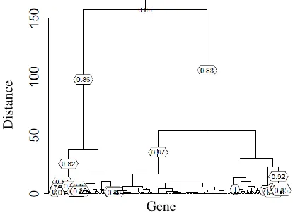
formation dataset had the numbers of genes as N=870, biological variables, T=6 and number of repetition, R=4. The sample result is shown in Figure 1. The result shows that the stability of the cluster were higher than 0.8 and there were more than 5 genes indicated. The number of samplings for the bootstrap procedure used to produce the dendrogram was 5, as shown in Figure 1.
Figure 1 Dendrogram of hierarchical clustering and cluster stability using Wood dataset
Figure 1 shows that there were a large number of nodes selected. This indicates that the dataset was a good quality dataset with low experimental and biological variability. However, there also exist less stability and irrelevant clusters. Figure 2 shows that the stability criterion of the clusters cannot be divided into smaller stable clusters. These clusters are the subtree in Figure 1. This subtree was chosen randomly among others subtrees. During the comparison, only the almost similar subtrees had been chosen for comparison.
Figure 2 Stable clusters which cannot be divided into smaller stable clusters. The value of the stability of the clusters is 0.87(shown with arrow)
Table 1 shows the result for original hierarchical clustering and hierarchical clustering which was incorporated with repeated measurement. The wood dataset had been analysed using different number of samplings for the bootstrap procedure.
Dis
tan
ce
Gene
Gene
Dis
tan
Table 1 Stability of gene clusters of wood formation dataset
Number of sampling for bootstrap procedure
Stability of the hierarchical gene clusters
5 0.87
10 0.86
15 0.88
20 0.87
25 0.89
30 0.84
35 0.89
40 0.89
45 0.87
50 0.88
As can be seen in Table 1, the differences between the stability of the gene clusters in wood formation dataset only had a small difference for all the different numbers of sampling for bootstraps procedure. The range for the stability was between 0.84 and 0.89. Therefore, the difference was only 0.05 even though the numbers of sampling for bootstrap procedure differed greatly, which were from 5 to 50.
The approximation made by averaging the repetitions did not have any significant impact to the stability. Therefore, this proves that the repeated measurement can be used in microarray dataset to validate the stability of gene clusters.
3.2 Bladder Cancer Dataset
The stage and outcome of bladder cancer stage and outcome were defined by using array based comparative genomic hybridization. This bladder cancer dataset contained N=2186 number of genes, T=14 conditions, and R=7 repetitions. Unfortunately, this dataset contained missing values. There were 10882 missing values in this dataset. To solve this problem, we used Bayesien Principal Component Analysis (BPCA) method to impute the missing values in the dataset.
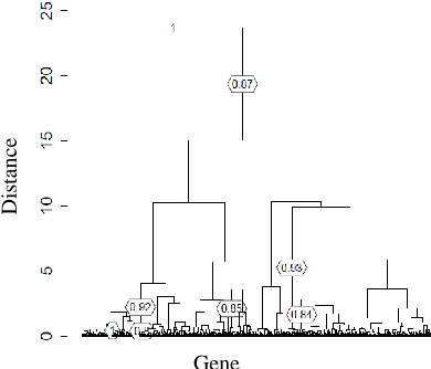
The result shown in Figure 3 for bladder cancer dataset, the stability of the cluster only indicated values higher than 0.8 and the number of genes was more than 5. The number of samplings for the bootstrap procedure used to produce the dendrogram was 5, as shown in Figure 3.
Figure 3 shows that only few clusters had stability more than 0.8. Thus, we can conclude that the hierarchy in this dataset in was less stable compared with the wood formation dataset. Therefore, the cluster must be considered attentively to prevent the selecting of non-significant clusters. Since the objective of this research was to validate the stability of the gene clusters, therefore, the stability of the cluster, which could not divide into, stable sub-clusters were chosen as the stability for comparison with each other. The arrow shown in Figure 3 denotes the clusters that had been chosen to compare their stability.
Figure 3 Dendrogram of hierarchical clustering of bladder cancer dataset
Table 2 Stability of gene clusters for bladder cancer dataset
Number of sampling for bootstrap procedure
Stability of the hierarchical gene clusters
5 0.84
10 0.85
15 0.83
20 0.85
25 0.82
30 0.84
35 0.83
40 0.82
45 0.85
50 0.84
Table 5.2 shows the stability of the gene cluster, which could not divide into stable sub-cluster. The difference between the gene clusters stability was low, only 0.03. The highest stability obtained this dataset was 0.85 while the lowest was 0.82. Since the difference did not differ much, therefore for this dataset, the objective to validation of gene clusters using repeated measurement with bootstrap procedure has been proven successful.
3.3 Yeast Galactose Dataset
This dataset was taken from the study done by Yeung, K. Y. et al. [13]. This dataset contained 205 numbers of genes, 20 biological conditions and 4 repeated measurements. The missing values were about 8% from the overall data. Therefore, data preprocessing was needed for this dataset by using BPCA method in MATLAB.
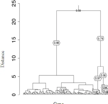
The dendrogram of the stability of yeast galactose dataset is shown in Figure 5. The dendrogram in Figure 5 only shows the stability of cluster which was greater than 0.8 and the minimum number of size cluster was greater than 5. Unfortunately, the dendrogram shown under this condition only indicated few numbers of nodes, and only few clusters were stable. This problem was overcome by using lower stability thresholdin, in which the stability threshold was changed to 0.6 instead of 0.8. The dendrogram produced using 0.6 stability threshold is shown in Figure 6.
Gene
Dis
tan
Figure 4 Result of yeast galactose dataset with 0.8stability threshold
Figure 5 Result of yeast galactose dataset with 0.6stability threshold
Figure 6 shows that the dendrogram contained larger number of nodes compared to the one in Figure 5. Since there are a large number of nodes in the dendrogram, therefore a zoom-in function was needed to carried out to observe the stability of the gene clusters. The zoom-in of the dendrogram is shown in Figure 7.
Figure 6 Zoom-in of the dendrogram
The arrow in Figure 7 points to the selected cluster that used its stability for comparison with each other, with different number of sampling for the bootstrap procedure. Table 3 shows the result of the stability.
Table 3 Stability of gene clusters for yeast galactose dataset
Number of sampling for bootstrap procedure
Stability of the hierarchical gene clusters
5 0.67
10 0.65
15 0.70
20 0.67
25 0.68
30 0.68
35 0.67
40 0.70
45 0.67
50 0.65
Table 3 shows that the highest stability was 0.7 while the lowest stability was 0.65. The difference between the highest and lowest stability was 0.05. Similar with other two datasets used in this research, the validation of hierarchical gene clusters using repeated measurement with bootstrap procedure has been proven successful although the value of stability for the dataset was lower.
3.4 Comparison Between the Datasets
This section discusses about the comparison between the dataset after the comparison of the stability within the same dataset. The main purpose of comparing the three datasets used in this research was to find out the best quality datasets among the three datasets. This can also be used to find which condition in the dataset that can be applied to obtain the best stability using the repeated measurement.
Table 4 Comparison of stability between the three datasets
Number of sampling for
bootstrap procedure
Wood formation
dataset
Bladder cancer dataset
Yeast galactose
dataset
5 0.87 0.84 0.67 10 0.86 0.85 0.65 15 0.88 0.83 0.70 20 0.87 0.85 0.67 25 0.89 0.82 0.68 30 0.84 0.84 0.68 35 0.89 0.83 0.67 40 0.89 0.82 0.70 45 0.87 0.85 0.67 50 0.88 0.84 0.65
Table 4 shows that the wood formation dataset had the highest stability among the three datasets and the yeast galactose dataset had the lowest stability. The numbers of genes in wood formation and bladder cancer dataset were almost the same. However, the wood formation dataset had higher stability. This shows that the wood formation dataset had a better quality, having lower biological or experimental condition compared with the bladder cancer dataset.
the yeast galactose dataset was the lowest therefore its stability was the lowest among the three datasets.
The quality of clustering with higher numbers of repeated measurement is usually higher [13]. The number of biological condition between bladder cancer and yeast galactose datasets was almost the same. However, since the bladder cancer and yeast galactose dataset had lower number of genes and number of repetitions compared to bladder cancer dataset, thus the stability of yeast galactoe dataset was lower than bladder cancer dataset.
In conclusion, the number of genes, number of biological condition and number of repetitions will influence the stability of the hierarchical gene cluster. In this research, wood formation has the best quality of dataset among the three datasets.
4.0 CONCLUSION
In conclusion, the hierarchical clustering technique applied in this research has successfully validated the clusters derived from hierarchical clustering. Different numbers of sampling in applying the bootstrap procedure for disturbance in the dataset also did not cause substantial changes onto the stability of the gene clusters.
Acknowledgement
We would like to express our gratitude to Universiti Teknologi Malaysia for supporting this research by granting us the UTM GUP research grants (Vote numbers: QJ130000.2507.01H29 and QJ130000.2523.00H67).
References
[1] E. Blaveri, J. L. Brewer, R. Roydasgupta, J. Fridlyand, S. DeVries, T.
Koppie, S. Pejavar, K. Mehta, P. Carroll, J. P. Simko, and F. M.
Waldman. 2005. Bladder Cancer Stage and Outcome by array-Based
Comparative Genomic Hybridization. Clin.Cancer Res. 11(7012).
[2] L. Brehelin, O. Gascuel and O. Martin. 2008. Using Repeated
Measuremnet to Validate Hierachical Gene Clsters. Gene Expression.
24(5): 682–688.
[3] S. Dudoit, and J. Fridlyand. 2002. A Prediction-based Resampling
Method for Estimating the Number of Cluster in a Dataset. Genome
Biology. 3(7): 1–21.
[4] M. B. Eisen, P. T. Spellman, P. O. Brown, and D. Botstein. 1998.
Cluster Analysis and Display of Genome-wide Expression Patterns.
Genetics. 95: 14863–14868.
[5] M. Hertzberg, H. Aspeborg, J. Schrader, A. Andersson, R. Erlandsson,
K. Blomqvist, R. Bhalerao, M. Uhlen, T. T. Teeri, J. Lundeberg, B. Sundberg, P. Nilsson, and G. Sandberg. 2001. A Transcriptional Roadmap to Wood Formation. PNAS. 98(25): 14732–14737.
[6] M. K. Kerr, and G. A. Churchill. 2001. Bootstrapping Cluster Analysis:
Assessing the Reliability of Conclusions from Microarray
Experiments. Proc. Natl. Acad. Sci. 98: 8961–8965.
[7] T. Lange, M. L. Braun, V. Roth, and J. M. Buhmann. 2003.
Stability-Based model Selection. Advance in Neural Information Processing
Systems. 15: 617–624.
[8] L. M. McShane, M. D. RadMacher, B. Freidlin, R. Yu, M. C. Li, and
R. Simon. 2002. Methods for Assessing Reproducibility of Clustering
Patterns Observed in Analyses of Microarray Data. Bioinformatics. 18:
1462–1469.
[9] M. Smolkin, and D. Ghosh. 2003. Cluster Stability scores for
Microarray Data in Cancer Studies. BMC Bioinformatics. 4.
[10] P. Tamayo, D. Slonim, J. Mesirov, Q. Zhu, S. Kitareewan, E. Dmitroovsky, E. S. Lander, and T. R. Golub. 1999. Interpreting Patterns of Gene Expression with Self-Organizing Maps: Methods and
Application to Hematopoietic Differentiation. Genetics. 96: 2907–
2912.
[11] S. Tavazoie, J. D. Hughes, M. J. Campbell, R. J. Cho, and G. M. Church. 1999. Systematic Determination of Genetic Network
Architecture. Nat. Genetic. 22: 281–285.
[12] K. Y. Yeung, D. R. Haynor, and W. L. Ruzzo. 2001. Validating
Clustering for Gene Expression Data. Bioinformatics. 17: 309–318.
[13] K. Y. Yeung, M. Medvedovix, and R. E. 2003. Bumgarner, Clsutering Gene Expression Data with Repeated measurement. Genome Biology. 4.
[14] K. Zhang, and H. Zhao. 2000. Assessing Reliability if Gene Clusters