Int. J. Advance. Soft Comput. Appl., Vol. 6, No.1 ,March 2014 ISSN 2074-8523; Copyright © SCRG Publication, 2014
Performance Improvement of
Least-Recently-Used Policy in Web Proxy Cache Replacement
Using Supervised Machine Learning
Waleed Ali1*, Sarina Sulaiman1, and Norbahiah Ahmad2
1
Soft Computing Research Group, Faculty of Computing, Universiti Teknologi Malaysia, 81310 Johor, Malaysia
email: [email protected], [email protected], [email protected] Abstract
Web proxy caching is one of the most successful solutions for improving the performance of Web-based systems. In Web proxy caching, Least-Recently-Used (LRU) policy is the most common proxy cache replacement policy, which is widely used in Web proxy cache management. However, LRU are not efficient enough and may suffer from cache pollution with unwanted Web objects. Therefore, in this paper, LRU policy is enhanced using popular supervised machine learning techniques such as a support vector machine (SVM), a naïve Bayes classifier (NB) and a decision tree (C4.5). SVM, NB and C4.5 are trained from Web proxy logs files to predict the class of objects that would be re-visited. More significantly, the trained SVM, NB and C4.5 classifiers are intelligently incorporated with the traditional LRU algorithm to present three novel intelligent Web proxy caching approaches, namely SVM-LRU, NB-LRU and C4.5-LRU. In the proposed intelligent LRU approaches, unwanted objects classified by machine learning classifier are placed in the middle of the cache stack used, so these objects are efficiently removed at an early stage to make space for new incoming Web objects. The simulation results demonstrated that the average improvement ratios of hit ratio achieved by SVM-LRU, NB-LRU and C4.5-LRU over LRU increased by 30.15%, 32.60% and 31.05 % respectively, while the average improvement ratios of byte hit ratio increased by 32.43%, 69.56% and 28.41%, respectively.
1 Introduction
The World Wide Web (Web) is the most common and significant service on the Internet. The Web contributes greatly to our life in many fields such as education, entertainment, Internet banking, remote shopping and software downloading. This has led to rapid growth in the number of Internet users, which resulting in an explosive increase in traffic or bottleneck over the Internet performance [1-2]. Consequently, this has resulted in problems during surfing some popular Web sites; for instance, server denials, and greater latency for retrieving and loading data on the browsers [3-5].
Web caching is a well-known strategy for improving the performance of Web-based system. In the Web caching, Web objects that are likely to be used in the near future are kept in a location closer to the user. Web caching mechanisms are implemented at three levels: client level, proxy level and original server level [6-7]. Proxy servers play key roles between users and Web sites in reducing the response time of user requests and saving network bandwidth. In this study, much emphasis is focused on the Web proxy caching because it is still the most common strategy used for caching Web pages[1-4, 8].
Due to cache space limitations, a Web proxy cache replacement is required to manage the Web proxy cache contents efficiently. In the proxy cache replacement, the proxy cache must effectively decide which objects are worth caching or replacing with other objects. The Web cache replacement is the core or heart of Web caching; hence, the design of efficient cache replacement algorithms is crucial for the success of Web caching mechanisms [4, 6-10]. So, the Web cache replacement algorithms are also known as Web caching algorithms [9].
In the Web cache replacement, a few important features or factors of Web objects, such as recency, frequency, size, cost of fetching the object from its origin server and access latency of object, can influence the performance of Web proxy caching [4, 6, 10-12]. These factors can be incorporated into the replacement decision for better performance.
The conventional Web cache replacement approaches consider just some factors and ignore other factors that have an impact on the efficiency of the Web caching [4, 9, 13-15]. Thus, the conventional Web proxy cache replacement policies are no longer efficient enough [4].
3 Performance Improvement of
Least-Recently-cache. Therefore, a large portion of objects, which are stored in the cache, are never requested again or requested after a long time. This leads to cache pollution, where the cache is polluted with inactive objects. This causes a reduction of the effective cache size and negatively affects the performance of Web proxy caching. Even if we can locate a large space for the proxy cache, this will be not helpful since the searching for a Web object in a large cache needs a long response time and an extra processing overhead. Furthermore, a consistency strategy is required to execute frequently to ensure the pages in the cache are the same as pages in the origin Web servers. This cause increase of network traffic, and more loads on the origin servers[1] .
This is motivation to adopt intelligent techniques for solving the Web proxy caching problems. The second motivation behind the development of intelligent approaches in Web caching is availability of proxy logs files that can be exploited as training data. In a Web proxy server, Web proxy logs file records activities of the users and can be considered as complete and prior knowledge of future access. Several research works have developed intelligent approaches that are smart and adaptive to the Web caching environment. These include adoption of supervised machine learning techniques [8-9, 14, 17-18], fuzzy systems [19], and evolutionary algorithms [12, 20-21] in Web caching and Web cache replacement. Recent studies have reported that the intelligent Web caching approaches based on supervised machine learning techniques are the most common, effective and adaptive Web caching approaches. A multilayer perceptron network (MLP) [9] and back-propagation neural network (BBNN) [8, 14], logistic regression (LR) [22] and multinomial logistic regression(MLR) [23], and adaptive neuro-fuzzy inference system(ANFIS)[15] have been utilized in Web caching. More details about intelligent Web caching approaches are given inour previous work [24]. Most of these studies have utilized an artificial neural network (ANN) in the Web caching although ANN performance is influenced by the optimal selection of the network topology and its parameters. Furthermore, ANN training may consume more time and require extra computational overhead. More significantly, integration of an intelligent technique in Web cache replacement is still a popular research subject.
This study proposes a concrete contribution to the field of Web proxy cache replacement. A new intelligent LRU cache replacement approaches with better performance are designed for use in Web proxy cache. The core of the proposed intelligent cache replacement approaches is to use common supervised machine learning techniques to predict whether Web objects would be needed again in the future. Then, classification decisions are utilized into the conventional LRU method determining what to remove first from the proxy cache.
The remaining parts of this paper are organized as follows. Background and related works are presented in Section 2. Principles of Web proxy caching and replacement are presented in Sections 2.2 and 2.3, while Section 2.4 describes machine learning classifiers used in this study, including support vector machines, decision trees and naïve Bayes classifier. A methodology for improving LRU replacement policy based on machine learning is illustrated in Section 3. Section 4 elucidates implementation and performance evaluation. Finally, Section 5 concludes the paper and discusses possible future works in this area.
2 Web Caching Background and Related Works
2.1 Overview
The term cache has French roots and means, literally, to store [33]. The idea of caching is used in memory architectures of modern computers for improving the performance of CPU speed. In a similar manner to caching in memory system, Web caching stores Web objects in anticipation of future requests. However, the Web caching significantly differs from traditional memory caching in several aspects such as the non-uniformity of Web object sizes, retrieval costs, and cacheability [33]. Significantly, the Web caching has several attractive advantages to Web users [34]. Firstly, the Web caching reduces user perceived latency. Secondly, the Web caching reduces network traffic and therefore reducing network costs for both content provider and consumers. Thirdly, the Web caching reduces loads on the origin servers. Finally, the Web caching increases reliability and availability of Web and application servers.
2.2 Web Proxy Caching
5 Performance Improvement of
Least-Recently-server behaves like both a client and a Least-Recently-server. It acts like a Least-Recently-server to clients, and like a client to servers. A proxy receives requests from clients, processes those requests, and then it forwards them to origin servers.
The Web proxy caching works on the same principle as the browser caching, but on a much larger scale. Unlike the browser cache that deals with only a single user, the proxy server serves hundreds or thousands of users in the same way. When a request is received, the proxy server checks its cache. If the object is available, the proxy server sends the object to the client. If the object is not available, or it has expired, the proxy server will request the object from the origin server and send it to the client. The requested objects are stored in the proxy’s local cache for future requests. Hence, the Web proxy caching plays the key roles between users and Web servers in reducing the response time of user requests and saving the network bandwidth.
The Web proxy caching is widely utilized by computer network administrators, technology providers, and businesses to reduce user delays and to reduce Internet congestion [1-3]. In this study, much emphasis are placed on Web proxy caching because it is still the most common strategy used for caching Web pages.
2.3 Web Proxy Cache Replacement
Three popular issues have a profound impact on Web proxy caching, namely cache consistency, cache pre-fetching, and cache replacement [34-36]. The cache consistency is to ensure the pages in the cache are the same as pages in the origin Web server. The pre-fetching is a technique for reducing user Web latency by preloading the Web object that is not requested yet by the user. In other words, the pre-fetching is a technique that downloads the probabilistic pages that are not requested by the user, but that could be requested soon by the same user [34]. The cache replacement refers to the process that takes place when the cache becomes full, and some objects must be removed to make space for new coming objects.
The Web proxy cache replacement plays an extremely important role in Web proxy caching. Hence, the design of efficient cache replacement algorithms is required to achieve highly sophisticated caching mechanism [4, 6-10]. The effective cache replacement algorithm is vital and has a profound impact on Web proxy cache management [7]. Therefore, this study pays attention to improvement of Web proxy cache replacement approaches. In general, cache replacement algorithms are also called Web caching algorithms [9].
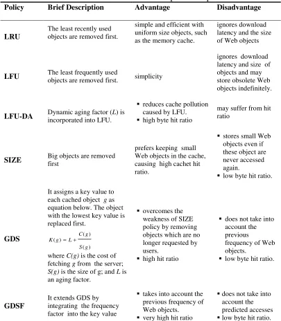
Most Web proxy servers are still based on conventional replacement policies for Web proxy cache management. In the proxy cache replacement, Least-Recently-Used (LRU), Least-Frequently-Least-Recently-Used (LFU), Least-Frequently-Least-Recently-Used-Dynamic- Least-Frequently-Used-Dynamic-Aging (LFU-DA), SIZE, Greedy-Dual-Size (GDS) and Greedy-Dual-Size-Frequency (GDSF) are the most common Web caching approaches, which still used in most of the proxy servers and software like squid software. These conventional Web caching methods form the basis of other Web caching algorithms [8, 14]. However, these conventional approaches still suffer from some limitations as shown in Table 1 [9, 37].
Table 1: Conventional Web cache replacement policies
Policy Brief Description Advantage Disadvantage
LRU
The least recently used objects are removed first.
simple and efficient with uniform size objects, such as the memory cache.
ignores download latency and the size of Web objects
LFU The least frequently used
objects are removed first. simplicity
ignores download latency and size of objects and may store obsolete Web objects indefinitely.
LFU-DA Dynamic aging factor (L) is
incorporated into LFU.
reduces cache pollution caused by LFU.
high byte hit ratio
may suffer from hit ratio
SIZE Big objects are removed
first
prefers keeping small Web objects in the cache, causing high cachet hit ratio.
stores small Web objects even if these object are never accessed again.
low byte hit ratio.
GDS
It assigns a key value to each cached object g as equation below. The object with the lowest key value is replaced first.
( ) ( )
( )
C g K g L
S g
= +
where C(g) is the cost of fetching g from the server;
S(g) is the size of g; and L is an aging factor.
overcomes the weakness of SIZE policy by removing objects which are no longer requested by users.
high hit ratio
does not take into account the previous
frequency of Web objects.
low byte hit ratio.
GDSF
It extends GDS by integrating the frequency factor into the key value
takes into account the previous frequency of Web objects.
very high hit ratio
does not take into account the predicted accesses
7 Performance Improvement of
Least-Recently-Least-Recently-Used (LRU) algorithm is one of the simplest and most common cache replacement approaches, which removes Web objects from the cache that have not been used for the longest period of time. In other words, LRU policy removes the least recently accessed objects first until there is sufficient space for the new objects. When a Web object is requested by user, the requested Web object is fetched from a server and placed at the top of the cache stack. Consequently, the cache stack pushes down the other objects in the stack so the object in the bottom of the cache stack is evicted from cache. Algorithm of the conventional LRU is shown in Fig. 1.
Fig. 1: The algorithm of conventional LRU proxy replacement policy The reason for the popularity of LRU in the Web proxy caching is the good performance of LRU when requests exhibit temporal locality, i.e., the Web object that have been requested in the recent past are likely to be requested again in the near future. However, if many objects stored by URL in the proxy cache are not requested again or requested after a long time, the cache usage is exploited inappropriately due to the cache pollution with unwanted objects. This causes a low performance of Web proxy caching.
As mentioned earlier, recency, frequency, size, cost of fetching the object and access latency of object are important features of Web objects, which play an essential role in making the wise decisions of Web proxy caching and replacement. In the conventional caching policies, only one factor is considered in cache replacement decision or few factors are combined using mathematical equation to predict revisiting of the Web objects in the future. These conventional approaches are not efficient enough and not adaptive to Web users' interests that change
Begin
For each Web object g requested by user
Begin
If g in cache
Begin
Cache hit occurs
Move g to top of the cache stack End
Else
Begin
Cache miss occurs Fetch g from origin server.
While no enough space in cache for g
Evict q such that q object in the bottom of the cache stack
Insert g at top of the cache stack
End End
continuously depending on rapid changes in Web environment. Therefore, alternative approaches are required in Web caching. Many Web cache replacement policies have been proposed to improve the performance of Web caching. However, it is challenging to have an omnipotent policy that performs well in all environments or for all time due to the preference of these factors is still based on the environments [6, 10]. Hence, there is a need for an intelligent and adaptive approach, which can effectively incorporate these factors into Web caching and replacement decisions.
2.4 Supervised machine learning
Machine learning involves adaptive mechanisms that enable computers to learn by example and learn from experience like human learning from experiences. The machine learning can be accomplished in a supervised or an unsupervised learning. In supervised learning, the data (observations) are labeled with pre-defined classes. It is like that a teacher gives the classes. On the other hand, unsupervised learning means that the system acts and observes the consequences of its actions, without referring to any predefined labels.
In this research, supervised machine learning techniques are proposed to improve the performance of Web proxy cache replacement. Support vector machine (SVM), naïve Bayes (NB) and decision tree(C4.5) are three popular supervised learning algorithms, which are identified as three of the most influential algorithms in data mining [25] and perform classifications more accurately and faster than other algorithms in a wide range of applications [26, 30].
Since SVM is formulated as a quadratic programming problem, there is a global optimum solution in SVM training. Besides, SVM is trained to maximize the margin, so the generalization ability can be maximized, especially when training data are scarce and linearly separable. In addition, SVM is robust to outliers because the margin parameter controls the misclassification error [38]. However, the generalization ability in SVM is still controlled by changing a kernel function and its parameters, and the margin parameter. Moreover, SVM may consume quite longer time compared to others in learning process, especially with large dataset. Hence, in addition to SVM, NB and C4.5 are also suggested for improving the performance of Web proxy cache replacement in this study. The NB and C4.5 are two of the most widely used and practical techniques for classification in many applications such as finance, marketing, engineering and medicine [29-32]. In addition to the good classification accuracy in many domains, the NB and C4.5 are efficient, easy to construct without parameters, and simple to understand and interpret [25, 27-28, 31].
2.4.1 Support vector machine
9 Performance Improvement of
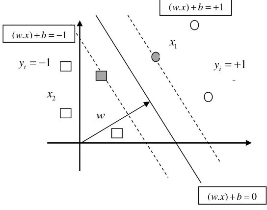
Least-Recently-hyperplane to do binary division (classification) with two classes, positive and negative samples. The SVM attempts to place hyperplane(solid line in Fig. 2) between the two different classes, and orient it in such a way that the margin (dotted lines in Fig. 2) is maximized. The hyperplane is oriented such that the distance between the hyperplane and the nearest data point in each class is maximal. The nearest data points are used to define the margins and are known as support vectors (SVs)(gray circle and square in Fig. 2). The hyperplane can be expressed as in Eq. (1)
Fig. 2: Classification of data by SVM
( . )
w x
+ =
b
0,
w R
∈
N,
b
∈
R
(1)where the vector w defines the boundary, x is the input vector of dimension N and
b is a scalar threshold. At the margins, where the SVs are located, the Eqs.(2) and (3) for positive class and negative class, respectively, are as follows:
( . )w x + =b 1 (2)
( . )w x + = −b 1 (3)
SVs correspond to the extremities of the data for a given class. Therefore, to classify any data point in either positive or negative class, the following decision Eq. (4) can be used:
( ) (( . ) )
f x =sign w x +b
(4) 1
x
1
i
y = +
2
x
1
i
y = −
w
( . )w x + = +b 1
( . )w x + = −b 1
The optimal hyperplane can be obtained as a solution to the following optimization problem.
Minimize
2
1
( )
2
t w
=
w
(5)Subject to
(( . )
) 1,
1,...,
i i
y
w x
+
b
≥
i
=
l
(6)where l is the number of training sets. The solution of the constrained optimization problem can be obtained using Eq.(7).
i i
w
=
∑
v x
(7)where xi are SVs obtained from training. Putting Eq. (7) in Eq. (4), the decision function is obtained in Eq. (8).
1
( )
( . )
l
i i i
f x
sign
v x x
b
=
=
+
∑
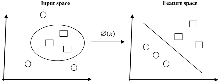
(8)However, for many real-life problems, it is not easy to find a hyperplane to classify the data such as nonlinearly separable data. The nonlinearly separable data is classified with the same principle of the linear case. However, the input data is only transformed from the original space into much higher dimensional space called the feature space. Then, a hyperplane can separate positive and negative examples in feature space as shown in Fig. 3. Thus, the decision function becomes as in Eq. (9).
Fig. 3: Transformation from input space to feature space
Input space Feature space
( )x
11 Performance Improvement of
Least-Recently-The transformation from input space to feature space space is relatively computation-intensive. Therefore, a kernel function can be used to perform this transformation and the dot product in a single step. This helps in reducing the computational load and at the same time retaining the effect of higher-dimensional transformation. The kernel function K x x( . )i j is defined as Eq.(10).
( . )
i j( ). (
i j)
K x x
= ∅
x
∅
x
(10)After substituting Eq. (10) in the decision function (9), the basic form of SVM is accordingly obtained as Eq. (11).
1
( )
( . )
l
i i
i
f x
sign
v K x x
b
=
=
+
∑
(11)The parameters vi are used as weighting factors to determine which of the input
vectors are support vectors. Several kernel functions can be used in SVM to solve different problems. In this study, RBF kernel given in Eq. (12) is used as kernel function in SVM training. The parameter γ represents the width of the RBF. In case there is an overlap between the classes with non-separable data, the range of parameters vi can be limited to reduce the effect of outliers on the boundary defined by SVs. For non-separable cases, the constraint becomes (0<vi<C). For separable cases, C is infinity while for non-separable cases, it may be varied, depending on the number of allowable errors in the trained solution: high C
permits few errors while low C allows a higher proportion of errors in the solution.
2
( , ) exp(
i j i j),
0
k x x
=
−
γ
x
−
x
γ
>
(12)2.4.2 Naïve Bayes classifier
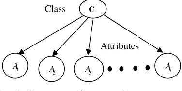
Naïve Bayes(NB) is very simple Bayesian network which has constrained structure of the graph [40]. In NB, all the attributes are assumed to be conditionally independent given the class label. The structure of the NB is illustrated in Fig. 4. In most of the data sets, the performance of the naïve Bayes classifier is surprisingly good even if the independence assumption between
1
( )
( ( ). ( ))
l
i i
i
f x
sign
v
x
x
b
=
=
∅
∅
+
attributes is unrealistic [40-41]. Independence between the features ignores any correlation among them.
Fig. 4: Structure of a naïve Bayes network
NB depends on probability estimations, called a posterior probability, to assign a class to an observed pattern. The classification can be expressed as estimating the class posterior probabilities given a test example d as shown in formula (13). The class with the highest probability is assigned to the example d.
Pr(
C
=
c
j| )
d
(13)Let A A1, 2,...,A/ /A be the set of attributes with discrete values in the data set D. Let
C be the class attribute with |C| values, c c1, 2,...,c/ /C . Given a test example
/ /
1 1,..., / /A A
d=< A =a A =a >, where ai is a possible value ofAi. The posterior
probability Pr(C=cj| )d can be expressed using the Bayes theorem as shown in Eq. (14).
/ / / /
/ /
1 1 / /
1 1 / /
1 1 / /
Pr( ,..., | )Pr( )
Pr( | ,..., )
Pr( ,..., )
A
A
A
A j j
j A
A
A a A a C c C c
C c A a A a
A a A a
= = = =
= = = =
= =
/ /
/ /
1 1 / /
/ /
1 1 / /
1
Pr( ,..., | ) Pr( )
Pr( ,..., | ) Pr( )
A
A
A j j
C
A k j
k
A a A a C c C c
A a A a C c C c
=
= = = =
=
= = = =
∑
(14)NB assumes that all the attributes are conditionally independent given the class
j
C=c as in Eq. (15),
/ /
/ /
1 1 / /
1
Pr( ,..., | ) Pr( | )
A
A
A j i i j
i
A a A a C c A a C c
=
= = = =
∏
= = (15)After putting (15) in (14), the decision function is obtained as shown in Eq. (16)
C
1
A
2
A A3 An
Class
13 Performance Improvement of
Least-Recently-/ Least-Recently-/
/ /
1
1 1 / / / /
1 1
Pr( ) Pr( | )
Pr( | ,..., )
Pr( ) Pr( | )
A
A
j i i j
i
j A C A
k i i k
k i
C c A a C c
C c A a A a
C c A a C c
=
= =
= = =
= = = =
= = =
∏
∑
∏
(16)In classification tasks, we only need the numerator of Eq. (16) to decide the most probable class for each example since the denominator is the same for each class. Thus we can decide the most probable class for given a test example using formula (17):
/ /
1
arg max Pr(
)
Pr(
|
)
j
A
j i i j
c i
c
C
c
A
a C
c
=
=
=
∏
=
=
(17)2.4.3 Decision tree
The most well-know algorithm in the literature for building decision trees is the C4.5 decision tree algorithm , which was proposed by Quinlan [42]. The basic concept of the C4.5 is as follow. The tree begins with a root node that represents the entire given dataset and it recursively splits the data into smaller subsets by testing for a given attribute at each node. The sub-trees denote the partitions of the original dataset that satisfy specified attribute value tests. This process typically continues until the subsets are pure. That means all instances in the subset fall into the same class, at which time the tree growing is terminated.
In the process of constructing the decision tree, the root node is first selected by evaluating each attribute on the basis of an impurity function to determine how well it alone classifies the training examples. The best attribute is selected and used to test at the root node of the tree. A descendant of the root node is created for each possible value of this selected attribute, and the training examples are sorted to the appropriate descendant node. The process is then repeated using the training examples associated with each descendant node to select the best attribute to test at that point in the tree.
3 A Methodology for Improving Least-Recently-Used
Replacement Policy Based on Supervised Machine
Learning
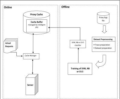
A framework for improving Least-Recently-Used replacement (LRU) policy in Web proxy cache replacement based on supervised machine learning classifiers is presented in Fig. 5.
Fig. 5: A framework for improving LRU replacement policy based on supervised machine learning classifiers
As shown in Fig. 5, the framework consists of two functional components: an online component and an offline component. The terms online and offline refer to interactive communications between the users and the proxy server. The offline component does not deal with the user directly, while online connections between the users and the proxy are established in the online component to retrieve the requested object from the proxy cache or the origin server. The offline component is responsible for training a machine learning classifier, while the intelligent LRU replacement approaches based on the trained classifier are utilized to effectively manage the Web proxy cache in the online component.
Proxy logs file
Training of SVM, NB or C4.5
SVM, NB or C4.5 classifier
Actual Requests
Cache Manager
Server Cache Buffer
managed by intelligent LRU Proxy Cache
Online Offline
Dataset Preprocessing
•Trace preparation
15 Performance Improvement of
Least-Recently-In the online component, when a user requests a Web page, the user communicates with the proxy, which directly retrieves the requested page from the proxy cache as shown in Fig. 5. However, sometimes the proxy cache miss occurs if the requested object is not in the proxy cache or not fresh. In a cache miss, the proxy server requests the object from the origin server and sends it back to the client. A copy of the requested object is replicated into the proxy cache to reduce the response time and the network bandwidth utilization in future requests. In some situations, a new coming object needs to be stored into the proxy cache; but the proxy cache is full of Web objects. In these cases, the proxy cache manger uses the proposed intelligent LRU replacement approaches to remove the unwanted Web objects in order to release enough space for the new coming object.
3.1
Training of supervised machine learning classifiers
The offline component is responsible for training the machine learning classifiers. In the proxy servers, information about the behaviours of groups of users in accessing many Web servers are recorded in files known as proxy logs files. The proxy logs files can be obtained from proxy servers located in various organizations or universities. The proxy logs files are considered a complete and prior knowledge of the users’ interests and can be utilized as training data to effectively predict the next Web objects.
4 Table 2: The inputs and their meanings
Input Meaning
1
x Recency of Web object access based on backward-looking sliding window
2
x Frequency of Web object accesses
3
x Frequency of Web object accesses based on backward-looking sliding window
4
x Retrieval time of Web object in milliseconds
5
x Size of Web object in bytes
6
x Type of Web object
1
x and x3are extracted based on a backward-looking sliding window in a similar manner to [8, 43] as shown in Eqs. (18) and (19). The backward-looking and forward-looking sliding windows of a request are the time before and after when the request was made.
( , ) ,
1
,
Max SWL T if object g was requested before
x
SWL otherwise
∆
=
(18)1 , 3 1
3
1 ,
x if T SWL
i x
i
otherwise
+ ∆ ≤
− =
(19)
where ∆T is the time in seconds since object g was last request , and SWL is sliding window length. If object g is requested for the first time, x3will be set to 1. In a similar way to Foong et al.[22], x6is classified into five categories: HTML with value 1, image with value 2, audio with value 3, video with value 4, application with value 5 and others with value 0.y is set based on the forward-looking sliding window. The value of y will be assigned to 1 if the object is re-requested again within the forward-looking sliding window. Otherwise, the target output will be assigned to 0. The idea is to use information about a Web object requested in the past to predict revisiting of such Web object within the forward-looking sliding window.
17 Performance Improvement of
Least-Recently-object requested by the user, either as Least-Recently-object would be revisited within the forward-looking sliding window or not.
As recommended by Hsu et al. [44], SVM is trained as follows: prepare and normalize the dataset, consider the RBF kernel, use cross-validation to find the best parameters C (margin softness) and γ (RBF width), use the best parameters to train the whole training dataset, and test. In SVM training, several kernel functions like polynomial, sigmoid and RBF can be used. However, in this study, RBF kernel function is used since it is the most often used kernel function and can achieve a better performance in many applications compared to other kernel functions [44]. After training, the obtained SVM uses Eq. (11) to predict the class of a Web objects either objects would be revisited again or not.
Regarding training of NB classifier, the NB classifier assumes that all attributes are categorical. Therefore, the numerical attributes need to be discretized into an interval in order to train or construct the NB classifier. In this study, the dataset is discretized by Minimum Description Length (MDL) given by Fayyad and Irani [45], and then the NB classifier is constructed depending on the finalized proxy dataset in order to classify Web objects as objects would be revisited again or not. In the training phase of NB classifier, it is only required to estimate the prior probabilities Pr(C = cj) and the conditional probabilities Pr(Ai =a Ci| =cj)from the proxy training dataset using Eqs. (20) and (21). Then, the NB classifier can predict class of a Web object using the formula (17), as explained in Section 2.4.2.
#
Pr(
)
#
j j
examples of class c
C
c
total examples
=
=
(20)#
Pr(
|
)
#
i i j
i i j
j
examples with A
a and class c
A
a C
c
examples of class c
=
=
=
=
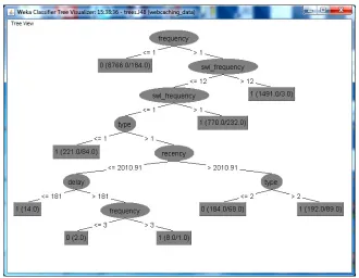
(21)Fig. 6: An example of building C4.5 decision tree for Web proxy dataset
3.2 The proposed intelligent LRU replacement approaches
based on machine learning classifiers
LRU policy is the most common proxy cache replacement policy among all the Web proxy caching algorithms [2-3, 8, 14]. However, LRU policy suffers from cold cache pollution, which means that unpopular objects remain in the cache for a long time. In other words, in LRU, a new object is inserted at the top of the cache stack. If the object is not requested again, it will take some time to be moved down to the bottom of the stack before removing it from the cache.
In order to reduce the cache pollution in LRU, the trained SVM, NB and C4.5 classifiers are combined with the traditional LRU to form three new intelligent LRU approaches known as SVM-LRU, NB-LRU and C4.5-LRU.
The proposed intelligent LRU approaches work as follows. When Web object g is requested by the user, the trained SVM, NB or C4.5 classifier predicts whether the class of that object would be revisited again or not. If object g is classified as an object would be re-visited again, object g is placed at the top of the cache stack. Otherwise, object g is placed in the middle of the cache stack used. As a result, the intelligent LRU approaches can efficiently remove unwanted objects at an early stage to make space for new Web objects.
19 Performance Improvement of
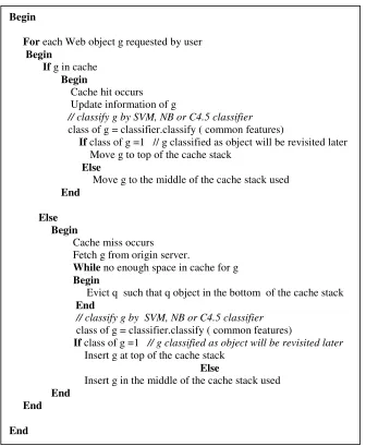
Least-Recently-be greatly improved by using the proposed intelligent LRU approaches. The algorithm of the proposed intelligent LRU is shown in Fig. 7.
Fig. 7: The algorithm of intelligent LRU approaches
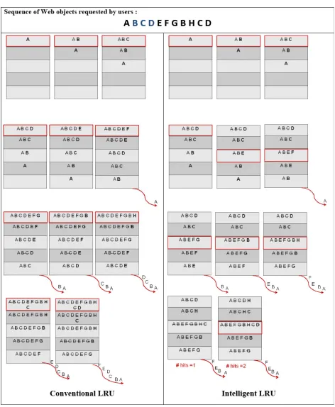
In order to understand the benefits of the proposed intelligent LRU, Fig. 8 illustrates an example of alleviating LRU cache pollution by using the intelligent LRU. Suppose that sequence of Web objects with fixed size is A B C D E F G B H C D requested by the users from left to right. The caching and removing of these objects using LRU policy and the proposed intelligent LRU are illustrated in Fig. 8.
Begin
For each Web object g requested by user
Begin
If g in cache
Begin
Cache hit occurs Update information of g
// classify g by SVM, NB or C4.5 classifier
class of g = classifier.classify ( common features)
If class of g =1 // g classified as object will be revisited later Move g to top of the cache stack
Else
Move g to the middle of the cache stack used
End
Else Begin
Cache miss occurs Fetch g from origin server.
While no enough space in cache for g
Begin
Evict q such that q object in the bottom of the cache stack
End
// classify g by SVM, NB or C4.5 classifier
class of g = classifier.classify ( common features)
If class of g =1 // g classified as object will be revisited later
Insert g at top of the cache stack
Else
Insert g in the middle of the cache stack used
End End
21 Performance Improvement of
Least-Recently-From Fig. 8, it can be observed that objects A, E, F, G, and H are visited only once, while the objects B, C and D are visited twice by user. In the traditional LRU policy, all Web objects are initially stored at the top of the cache, so these objects need longer time to move down to the bottom of the cache (where least recently used objects are stored) for removal from the cache.
By contrast, the proposed intelligent LRU (see Fig. 8) stores the preferred objects B, C and D at the top of the cache if the machine learning classifier predicts correctly revisiting of B, C and D again. On the other hand, if objects A, E, F, and G are properly classified as objects would not be re-visited soon, then these objects will be stored in the middle of the proxy cache used. Therefore, these objects A, E, F and G move down to the bottom of the cache shortly. Hence, the un-preferred objects are removed in a short time by the intelligent LRU to make space for new Web objects.
From the above example, it can be noted that the proposed intelligent LRU approaches efficiently remove unwanted objects early to make space for new Web objects. Therefore, the cache pollution is lessened and the available cache space is exploited efficiently. Moreover, the hit ratio and byte hit ratio can be improved successfully.
4 Performance Evaluation and Discussion
4.1 Raw data collection and pre-processing
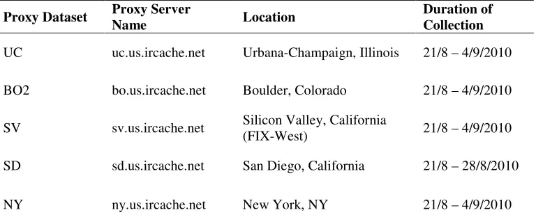
The proxy datasets or the proxy logs files were obtained from five proxy servers located in the United States from the IRCache network and covered fifteen days [46]. Four proxy datasets (BO2, NY, UC and SV) were collected between 21st August and 4th September, 2010, while SD proxy dataset was collected between 21st and 28th August, 2010. In this study, the proxy logs files of 21st August, 2010 were used in the training phase, while the proxy logs files of the following days were used in the simulation to evaluate the proposed intelligent Web proxy cache replacement approaches against existing works (see Table 3).
Each line in the proxy logs file represents access proxy log entry, which consists of the ten following fields: timestamp, elapsed time, client address, log tag and HTTP code, size request method, URL, user identification, hierarchy data and hostname and content type.
Table 3: Proxy datasets used for evaluating the proposed intelligent caching approaches
Proxy Dataset Proxy Server
Name Location
Duration of Collection
UC uc.us.ircache.net Urbana-Champaign, Illinois 21/8 – 4/9/2010
BO2 bo.us.ircache.net Boulder, Colorado 21/8 – 4/9/2010
SV sv.us.ircache.net Silicon Valley, California
(FIX-West) 21/8 – 4/9/2010
SD sd.us.ircache.net San Diego, California 21/8 – 28/8/2010
NY ny.us.ircache.net New York, NY 21/8 – 4/9/2010
Parsing: This involves identifying the boundaries between successive records in log files as well as the distinct fields within each record.
Filtering: This includes elimination of irrelevant entries such as un-cacheable requests (i.e., queries with a question mark in the URLs and cgi-bin requests) and entries with unsuccessful HTTP status codes. We only consider successful entries with 200 status codes.
Finalizing: This involves removing unnecessary fields. Moreover, each unique URL is converted to a unique integer identifier for reducing time of simulation.
4.2 Raw data collection and pre-processing
4.2.1 Training phase
23 Performance Improvement of
Least-Recently-Once the datasets were properly prepared, the machine learning techniques were implemented using MATLAB and WEKA. The SVM model was trained using the libsvm library [47]. The generalization capability of SVM is controlled through a few parameters such as the term C and the kernel parameter like RBF widthγ . To decide which values to choose for parameter C andγ , a grid search algorithm was implemented as suggested by Hsu et al. [44]. The parameters that obtain the best accuracy using a 10-fold cross validation on the training dataset were retained. Next, a SVM model was trained depending on the optimal parameters to predict and classify the Web objects whether the objects would be re-visited or not. Regarding C4.5 training, a J48 learning algorithm was used, which is a Java re-implementation of C4.5 and provided with WEKA tool. The default values of parameters and settings were used as determined in WEKA. In NB training, the datasets were discretized using a MDL method suggested by Fayyad and Irani [45] with default setup in WEKA. Once the training dataset was prepared and discretized, NB was trained using WEKA as well. In WEKA, a NB classifier is available in the Java class “weka.classifiers.bayes.NaiveBayes”.
4.2.2 Classifiers evaluation
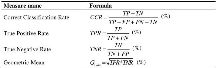
The main measure for evaluating a classifier is the correct classification rate (CCR), which is the number of correctly classified examples in the dataset divided by the total number of examples in the dataset. In some situations, CCR alone is insufficient for measuring the performance of a classifier, e.g., when the data is imbalanced. Therefore, some accurate measures of the classification evaluation are extracted from a confusion matrix shown in Table 4.
Table 4: Confusion matrix for a two-class problem
Predicted Positive Predicted Negative
Actual Positive True Positive (TP) False Negative (FN)
Actual Negative False Positive (FP) True Negative (TN)
Table 5: The measures used for evaluating performance of machine learning classifiers
Measure name Formula
Correct Classification Rate CCR TP TN
TP FP FN TN
+ =
+ + + (%)
True Positive Rate TPR TP TP FN
=
+ (%)
True Negative Rate TNR TN
TN FP
=
+ (%)
Geometric Mean Gmean= TPR TNR* (%)
study that the training datasets are imbalanced since many Web objects are visited just one time by the users. Therefore, like several research works [23, 48-49], CCR, true positive rate (TPR) or sensitivity, true negative rate (TNR) or specificity, and geometric mean (GM) are used in this study to evaluate the classifiers performance as shown in Table 5.
In this paper, both hold-out validation and n-fold cross validation were used in evaluating the supervised machine learning algorithms. In hold-out validation, each proxy dataset was randomly divided into training data (70%) and testing data (30%). In addition, 10-fold cross validation was used in evaluating the supervised machine learning algorithms since it is commonly used by many researchers. In order to benchmark the SVM, NB and C4.5, they were compared to both back-propagation neural network (BPNN) and adaptive neuro-fuzzy inference system (ANFIS). This is due to the fact that BPNN and ANFIS have good performance in Web caching area in pervious works [8-9, 14-15, 17-18, 37]. In addition, the SVM, NB and C4.5 were also compared with BPNN as used in the existing caching approach NNPCR-2 [8].
Tables 6 and 7 show comparisons between the performance measures of SVM, NB, C4.5, BPNN, ANFIS and NNPCR-2 for the five proxy datasets in testing phase using hold-out and 10-fold cross-validations. In Tables 6 and 7, the best and the worst values of the measures are highlighted in bold font and underline font, respectively. In hold-out validation shown in Table 6, SVM, NB and C4.5 achieved the averages of CCR around 94.33%, 94.43% and 94.55%, while BPNN, ANFIS, and NNPCR-2 achieved the averages of CCR around 87.39%, 93.93% and 86.37% respectively. In 10-fold cross-validation shown in Table 7, SVM, NB and C4.5 achieved the averages of CCR around 94.53%, 94.59% and 94.79% respectively, while BPNN and ANFIS, and NNPCR-2 achieved the averages of CCR around 87.79%, 93.72% and 85.53% respectively. As can be seen from Tables 6 and 7, SVM, NB, C4.5 and ANFIS produced competitive performances in terms of CCR. However, it is obvious that SVM, NB and C4.5 achieved higher CCR when compared to the CCR of BPNN and NNPCR-2. This was due to the fact that BPNN training could be trapped in a local minimum, while there is a global optimum solution in SVM training.
25 Performance Improvement of
Least-Recently-susceptible to imbalanced data when compared to BPNN and ANFIS, as can be observed from Tables 6 and 7. This indicated that SVM, NB and C4.5 had better GM and TPR when compared to others.
Table 6: Performance measures of machine learning algorithms in hold-out validation
BO2 NY UC SV SD Average
SVM
CCR 95.30 91.19 95.54 93.76 95.84 94.326
TPR 86.41 91.95 92.76 91.16 89.17 90.29
TNR 96.16 90.95 95.93 94.36 96.83 94.846
GM 91.15 91.45 94.33 92.97 92.92 92.564
NB
CCR 95.34 91.35 95.74 93.78 95.93 94.428
TPR 82.14 88.22 86.9 82.39 88.94 85.718
TNR 96.61 92.34 96.95 96.95 96.98 95.966
GM 89.08 90.26 91.79 89.38 92.87 90.676
C4.5
CCR 95.68 91.26 95.88 94.02 95.91 94.55
TPR 68.54 89.36 78.27 87.87 83.81 81.57
TNR 98.30 91.86 98.29 95.74 97.72 96.382
GM 82.08 90.60 87.71 91.72 90.50 88.522
BPNN
CCR 94.08 75.90 90.36 87.95 88.65 87.388
TPR 32.62 0.00 20.07 45.69 12.77 22.23
TNR 100.00 100.00 99.99 99.73 99.98 99.94
GM 57.12 0.00 44.79 67.50 35.73 41.028
ANFIS
CCR 95.30 91.23 94.75 92.94 95.43 93.93
TPR 61.55 84.94 62.46 76.53 74.77 72.05
TNR 98.56 93.22 99.17 97.52 98.52 97.398
GM 77.89 88.98 78.71 86.39 85.83 83.56
NNPCR-2
CCR 91.41 76.25 90.05 87.11 87.01 86.366
TPR 7.77 2.49 17.44 40.92 0 13.724
TNR 99.48 99.67 100 99.99 100 99.828
Table 7: Performance measures of machine learning algorithms in 10-fold cross validation
BO2 NY UC SV SD Average
SVM
CCR 95.5 91.7 95.58 93.88 95.97 94.526
TPR 87.61 92.57 92.62 92.02 89.28 90.82
TNR 96.27 91.43 95.98 94.39 96.95 95.004
GM 91.82 92 94.29 93.2 93.04 92.87
NB
CCR 95.57 91.79 95.71 93.86 96 94.586
TPR 83.46 88.48 87.73 82.72 88.83 86.244
TNR 96.76 92.84 96.79 96.89 97.06 96.068
GM 89.84 90.63 92.15 89.52 92.85 90.998
C4.5
CCR 95.6 92.19 96.03 94.08 96.03 94.786
TPR 67.09 83.5 80.7 86.7 84.23 80.444
TNR 98.38 94.95 98.1 96.09 97.77 97.058
GM 81.2 89.03 88.97 91.27 90.75 88.244
BPNN
CCR 92.21 80.41 90.15 88.06 88.11 87.788
TPR 12.64 21.19 18.23 45.73 7.91 21.14
TNR 99.97 99.25 99.84 99.54 99.92 99.704
GM 26.31 45.5 35.61 64.32 22.47 38.842
ANFIS
CCR 94.67 91.11 95.13 92.38 95.32 93.722
TPR 56.9 84.16 65.26 74.55 73.68 70.91
TNR 98.37 93.32 99.16 97.22 98.51 97.316
GM 74.81 88.62 80.44 85.13 85.19 82.838
NNPCR-2
CCR 91.28 76.42 89.34 83.32 87.29 85.53
TPR 2.36 3.41 10.74 22.43 1.35 8.058
TNR 99.95 99.65 99.92 99.84 99.94 99.86 GM 6.87 16.82 27.97 46.44 6.33 20.886
27 Performance Improvement of
Least-Recently-Table 8: The computational time for training the supervised machine learning algorithms in hold-out validation
Dataset Training Time(seconds)
SVM NB C4.5 BPNN ANFIS NNPCR-2
BO2 9.11 0.12 0.36 146.59 41436.63 69.50
NY 69.41 0.35 0.85 316.34 89057.09 153.62
UC 280.30 1.59 3.36 701.18 202033.64 342.61
SV 52.20 0.33 0.69 303.40 85753.53 153.30
SD 291.51 1.32 2.90 693.36 205294.87 345.068
Average 140.506 0.742 1.632 432.174 124715.2 212.8196
Table 9: The computational time for training supervised machine learning algorithms in 10-fold cross validation
Dataset Training Time(seconds)
SVM NB C4.5 BPNN ANFIS NNPCR-2
BO2 14.55 0.14 0.26 188.26 65507.18 79.75
NY 126.92 0.51 1.29 385.85 120657.97 167.44
UC 500.15 1.96 4.32 865.07 284267.57 376.03
SV 100.02 0.51 1.05 375.62 115745.14 163.67
SD 436.76 1.84 4.55 851.26 281538.43 764.33
Average 235.68 0.992 2.294 533.212 173543.3 310.244
4.3 Evaluation of intelligent LRU approaches
4.3.1 Web proxy cache simulation
4.3.2 Performance Measures
The hit ratio (HR) and byte hit ratio (BHR) are the most widely used metrics in evaluating the performance of Web caching [8-10, 14]. HR is defined as the percentage of requests that can be satisfied by the cache. Note that HR only indicates how many requests hit and does not indicate how much bandwidth can be saved. BHR is the number of bytes satisfied from the cache as a fraction of the total bytes requested by the user. BHR represents the saved network bandwidth achieved by caching approach.
It is important to note that HR and BHR work in somewhat opposite ways. It is very difficult for one strategy to achieve the best performance for both metrics [4, 8, 50-51]. This is due to the fact that the strategies that increase HR typically give preference to small objects, but these strategies tend to decrease BHR by giving less consideration to larger objects. On the contrary, the strategies that do not give preference to small objects tend to increase BHR at the expense of HR.
4.3.3 Performance measures of infinite cache
An infinite cache is a cache with enough space to store all requested objects without the need to replace any object. The infinite cache size is defined as the total size of all unique requests. Therefore, it is unnecessary to consider any replacement policy for an infinite cache. In an infinite cache, HR and BHR reach their maximum values.
In reality, the caches cannot be designed as infinite. A replacement policy is needed when the cache is full, and this has a great effect on the performance of Web caching systems. However, in our simulation the infinite cache is required to determine the maximum cache size in the simulator, which represents the stop point during the simulation. Table 10 shows some statistical information for the maximum HR and BHR for the five proxy datasets used in the simulation.
Table 10: Statistics for different proxy datasets used in simulation
BO2 NY UC SV SD
#Total requests 1210693 3248452 8891764 2496001 29871204
#Cacheable
requests 594989 1518232 2827904 1194098 6059349
#Cacheable bytes 23204930341 68402036319 469362584083 48043794224 230326816876
#Unique requests 530192 1144885 2402406 1012355 5284441
Total size of unique
requests ( bytes) 18690093450 56147903761 156538171752 38364029432 190539902251
#Hits 64797 373347 425498 181743 774908
#Byte Hits 4514836891 12254132558 312824412331 9679764792 39786914625
Max HR(%) 10.89 24.59 15.05 15.22 12.79
29 Performance Improvement of
Least-Recently-4.3.4 Impact of cache size on performance measures
By using the WebTraff simulator, the proposed SVM-LRU, NB-LRU and C4.5-LRU approaches were compared with the conventional C4.5-LRU algorithm across the five proxy datasets: BO2, NY, UC, SV, and SD. For each dataset, the Web proxy caching algorithms were simulated with varying limits of the cache size starting at 1 MB to 32 GB in order to determine the impact of cache size on the performance measures. The simulation was stopped at 32 GB since the performances of all algorithms became stable and close to the maximum level achieved for a cache of infinite size.
Figs. 9 and 10 show the HR and BHR of different policies for the five proxy datasets with varying cache sizes. As can be seen in Figs. 9 and 10, when the cache size increased, the HR and BHR also provided a boost for all algorithms. However, the percentage of increase was reduced when the cache size increased. When the cache size was close to the size of the infinite cache, the performance became stable and close to its maximum level. On the contrary, when the cache size was small, the replacement of objects was frequently required. Hence, the effect of the performance of replacement policy was clearly noted.
As can be observed from Figs. 9 and 10, SVM-LRU, NB-LRU and C4.5-LRU produced better performances in terms of HR and BHR when compared to the conventional LRU, especially with small sizes of cache. This was mainly due to the capability of intelligent LRU approaches for storing the preferred objects for longer time. Depending on classification decisions, the preferred objects were placed at the top of cache stack, so these objects took longer time to move down to the bottom of the cache stack where they would be removed from the cache. On the other hand, the unwanted objects were removed from the proxy cache at earlier stage. This eventually reduced the cache pollution. Consequently, the performance in terms of HR and BHR of LRU was improved by using SVM-LRU, NB-LRU and C4.5-LRU.
For comparison of intelligent LRU approaches with each other, SVM-LRU, NB-LRU and C4.5-NB-LRU achieved competitive HR in the different cache sizes across the five proxy datasets, as can be seen from Fig. 9. This was due to the equivalent capability of intelligent classifiers to predict the classes of objects, whether objects would be re-visited or not. In general, C4.5-LRU and SVM-LRU achieved slightly higher HR when compared to NB-LRU. In terms of BHR, Fig. 10 shows that SVM-LRU and NB-LRU achieved better BHR when compared to C4.5-LRU in different proxy cache sizes for most the proxy datasets.
Furthermore, the performance in terms of HR and BHR could be influenced by changing the sizes of the proxy cache between 1 MB and 32 GB.
In order to clarify the benefits of the intelligent LRU approaches, the improvement ratio (IR) of the performance in terms of HR and BHR in each particular cache size can be calculated using Eq. (22).
( )
100 (%)
PM CM
IR
CM
−
= × (22)
where IR is the percent of improvement in terms of HR or BHR achieved by the proposed method (PM) over the conventional method (CM). CM refers the performance in terms of HR or BHR of the conventional LRU. PM represents the performance in terms of HR or BHR of the proposed intelligent LRU: SVM-LRU, NB-LRU and C4.5-LRU.
The average IRs of the performances in terms of HR and BHR of the intelligent LRU approaches for the five proxy datasets in each particular cache are concluded and summarized in Table 11. In Table 11 , the highest and the lowest values of the average IRs are highlighted in bold and underline fonts, respectively.
Table 11: The average IRs (%) achieved by intelligent LRU approaches over conventional LRU method
Cache Size (MB)
Average IR of SVM-LRU Over LRU (%)
Average IR of NB-LRU Over LRU (%)
Average IR of C4.5-LRU Over LRU (%)
HR BHR HR BHR HR BHR
1 30.15 20.84 32.596 22.966 31.046 20.84
2 23.26 27.05 23.326 57.776 24.14 28.408
4 13.988 29.846 11.722 69.564 15.43 28.118
8 12.318 24.208 12.078 33.312 14.648 25.946
16 9.692 17.58 10.05 21.468 11.452 20.216
32 8.294 14.44 8.408 14.604 9.852 15.832
64 10.408 32.434 11.244 23.454 11.904 22.802
128 5.08 15.054 4.736 10.318 6.568 10.336
256 4.974 7.596 4.174 6.188 6.222 6.938
512 5.804 5.316 5.206 5.066 6.878 5.276
1024 5.65 2.874 5.142 2.898 6.588 2.932 2048 4.422 0.794 3.846 0.794 5.224 1.07 4096 2.87 0.81 2.426 1.104 3.376 0.81
31 Performance Improvement of
H it R a t io (% ) Cache Size(MB)
Hit Ratio for BO2 Dataset LRU SVM-LRU NB-LRU C4.5-LRU H it R a t io (% ) Cache Size(MB) Hit Ratio for NY Dataset
LRU SVM-LRU NB-LRU C4.5-LRU H it R a t io (% ) Cache Size(MB)
Hit Ratio for UC Dataset
LRU SVM-LRU NB-LRU C4.5-LRU H it R a t io (% ) Cache Size(MB)
Hit Ratio for SV Dataset
LRU SVM-LRU NB-LRU C4.5-LRU H it R a ti o (% ) Cache Size(MB)
Hit Ratio for SD Dataset LRU
SVM-LRU
NB-LRU
C4.5-LRU
33 Performance Improvement of
Least-Recently-B y t e H it R a t io (% ) Cache Size(MB)
Byte Hit Ratio for BO2 Dataset
LRU SVM-LRU NB-LRU C4.5-LRU B y t e H it R a t io (% ) Cache Size(MB)
Byte Hit Ratio for NY Dataset
LRU SVM-LRU NB-LRU C4.5-LRU B y t e H it R a t io ( % ) Cache Size(MB)
Byte Hit Ratio for UC Dataset
LRU SVM-LRU NB-LRU C4.5-LRU B y t e H it R a t io (% ) Cache Size(MB)
Byte Hit Ratio for SV Dataset
LRU SVM-LRU NB-LRU C4.5-LRU B yt e H it R at io (% ) Cache Size(MB)
Byte Hit Ratio for SD Dataset
LRU SVM-LRU NB-LRU C4.5-LRU
5 Conclusion and Future Works
In order to improve the performance of Web proxy caching, this paper presented a framework for improving the conventional LRU replacement policy based on supervised machine learning classifiers. The framework consisted of two functional components: online and offline components. In the offline component, SVM, NB and C4.5 were intelligently trained from proxy logs files to classify the contents of Web proxy cache. In the online component, the trained SVM, NB and C4.5 classifiers were effectively utilized to improve the performance of the conventional LRU policy, which widely used in Web proxy cache replacement. In particular, the conventional LRU technique was extended by efficiently integrating the classification decisions made by the trained SVM, NB and C4.5 classifiers into cache replacement decisions to obtain more efficient and intelligent SVM-LRU, NB-LRU and C4.5-LRU approaches. For testing and evaluating the proposed proxy caching methods, the proxy logs files were obtained from several proxy servers located around the United States of the IRCache network, which are the most common proxy datasets used in the research of Web proxy caching. The experimental results showed that SVM, NB and C4.5 achieved a better accuracy and a much faster than BPNN and ANFIS. Furthermore, the proposed intelligent LRU approaches were evaluated by trace-driven simulation and compared with the conventional LRU policy. The simulation results revealed that the proposed intelligent LRU approaches considerably improved the performance in terms of hit ratio and byte hit ratio of the conventional LRU on a range of datasets.
There are some limitations in this study. One of the limitations is that the classifiers in the proposed intelligent LRU approaches were trained once and then were used to predict the classes of Web object over the next one or two weeks. A regular retraining of classifiers would ensure that the proposed intelligent LRU approaches become more efficient and adaptive. Another limitation is the preparation of the target outputs in training phase that required extra computational overhead when looking for the future requests. Therefore, unsupervised machine learning algorithms can be used for enhancing the performance of Web caching policies since the unsupervised algorithms do not need any preparation for the target outputs. Furthermore, other intelligent classifiers can be also utilized to improve both the hit ratio and the byte hit ratio of traditional Web caching policies.
ACKNOWLEDGEMENTS.