Networks
(Revised August 2005)
Donggang Liu
The University of Texas at Arlington and
Peng Ning
North Carolina State University and
Wenliang Kevin Du Syracuse University
Many sensor network applications require sensors’ locations to function correctly. Despite the recent advances, location discovery for sensor networks inhostile environmentshas been mostly
overlooked. Most of the existing localization protocols for sensor networks are vulnerable in hostile environments. The security of location discovery can certainly be enhanced by authentication. However, the possible node compromises and the fact that location determination uses certain physical features (e.g., received signal strength) of radio signals make authentication not as effec-tive as in traditional security applications. This paper presents two methods to tolerate malicious attacks against beacon-based location discovery in sensor networks. The first method filters out malicious beacon signals on the basis of the “consistency” among multiple beacon signals, while the second method tolerates malicious beacon signals by adopting an iteratively refined voting scheme. Both methods can survive malicious attacks even if the attacks bypass authentication, provided that the benign beacon signals constitute the majority of the beacon signals. This paper also presents the implementation of these techniques on MICA2 motes running TinyOS, and the evaluation through both simulation and field experiments. The experimental results demonstrate that the proposed methods are promising for the current generation of sensor networks.
Categories and Subject Descriptors: C.2.0 [Computer-Communication Networks]: General—Security and pro-tection; C.2.1 [Computer-Communication Networks]: Network Architecture and Design—Wireless communi-cation
General Terms: Security, Design, Algorithms
Additional Key Words and Phrases: Sensor Networks, Security, Localization
This work is supported by the National Science Foundation (NSF) under grants CNS-0430223 and CNS-0430252. A preliminary version of this paper appeared in the Proceedings of The Fourth International Symposium on Information Processing in Sensor Networks (IPSN ’05), pages 99 – 106, April 2005.
Permission to make digital/hard copy of all or part of this material without fee for personal or classroom use provided that the copies are not made or distributed for profit or commercial advantage, the ACM copyright/server notice, the title of the publication, and its date appear, and notice is given that copying is by permission of the ACM, Inc. To copy otherwise, to republish, to post on servers, or to redistribute to lists requires prior specific permission and/or a fee.
c
1. INTRODUCTION
Recent technological advances have made it possible to develop distributed sensor net-works consisting of a large number of low-cost, low-power, and multi-functional sensor nodes that communicate in short distances through wireless links [Akyildiz et al. 2002]. Such sensor networks are ideal candidates for a wide range of applications such as health monitoring, data acquisition in hazardous environments, and military operations. The de-sirable features of distributed sensor networks have attracted many researchers to develop protocols and algorithms that can fulfill the requirements of these applications (e.g., [Perrig et al. 2001; Hill et al. 2000; Gay et al. 2003; Niculescu and Nath 2001; Intanagonwiwat et al. 2003; Newsome and Song 2003; Akyildiz et al. 2002]).
Sensors’ locations play a critical role in many sensor network applications. Not only do applications such as environment monitoring and target tracking require sensors’ location information to fulfill their tasks, but several fundamental techniques developed for wireless sensor networks also require sensor nodes’ locations. For example, in geographical routing protocols (e.g., GPSR [Karp and Kung 2000] and GEAR [Yu et al. 2001]), sensor nodes make routing decisions at least partially based on their own and their neighbors’ locations. As another example, in some data-centric storage applications such as GHT [Ratnasamy et al. 2002; Shenker et al. 2002], storage and retrieval of sensor data highly depend on sen-sors’ locations. Indeed, many sensor network applications will not work without sensen-sors’ location information.
A number of location discovery protocols (e.g., [Savvides et al. 2001; Savvides et al. 2002; Niculescu and Nath 2003a; Nasipuri and Li 2002; Doherty et al. 2001; Bulusu et al. 2000; Niculescu and Nath 2003b; Nagpal et al. 2003; He et al. 2003]) have been proposed for wireless sensor networks in recent years. These protocols share a common feature: They all use some special nodes, called beacon nodes, which are assumed to know their own locations (e.g., through GPS receivers or manual configuration). These protocols work in two stages. In the first stage, non-beacon nodes receive radio signals called beacon
sig-nals from the beacon nodes. The packet carried by a beacon signal, which we call a beacon packet, usually includes the location of the beacon node. The non-beacon nodes then
esti-mate certain measurements (e.g., distance between the beacon and the non-beacon nodes) based on features of the beacon signals (e.g., received signal strength indicator (RSSI), time difference of arrival (TDoA)). We refer to such a measurement and the location of the corresponding beacon node collectively as a location reference. In the second stage, a sensor node determines its own location when it has enough number of location references from different beacon nodes. A typical approach is to consider the location references as constraints that a sensor node’s location must satisfy, and estimate it by finding a math-ematical solution that satisfies these constraints with minimum estimation error. Existing approaches either employ range-based methods [Savvides et al. 2001; Savvides et al. 2002; Niculescu and Nath 2003a; Nasipuri and Li 2002; Doherty et al. 2001], which use the exact measurements obtained in stage one, or range-free ones [Bulusu et al. 2000; Niculescu and Nath 2003b; Nagpal et al. 2003; He et al. 2003; Lazos and Poovendran 2004], which only need the existences of beacon signals in stage one.
Despite the recent advances, location discovery for wireless sensor networks in hostile
environments, where there may be malicious attacks, has been mostly overlooked. Many
beacon node nb
(x, y)
attacking node na
n
(x’, y’)
I’m nb; my location is (x, y)
(a) Masquerade beacon nodes
malicious beacon node nb
(x, y)
n I’m nb; my location
is (x’, y’)
(b) Compromised beacon nodes
beacon node nb
(x, y) attacking node na
n
(x’, y’)
I’m nb; my location is
(x, y)
replay “I’m nb; my
location is (x, y)”
(c) Replay attack
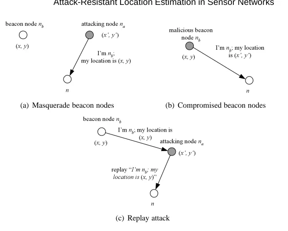
Fig. 1. Attacks against location discovery schemes
pretending to be valid beacon nodes (Figure 1(a)), compromising beacon nodes (Figure 1(b)), or replaying the beacon packets that he/she intercepted in different locations (Figure 1(c) ). In either of the above cases, non-beacon nodes will determine their locations incor-rectly. In either of these cases, non-beacon nodes will determine their locations incorincor-rectly. Without protection, an attacker may easily mislead the location estimation at sensor nodes and subvert the normal operation of sensor networks. The security of location discovery can certainly be enhanced by authentication. Specifically, each beacon packet should be authenticated with a cryptographic key only known to the sender and the in-tended receivers, and a non-beacon node accepts a beacon signal only when the beacon packet carried by the beacon signal can be authenticated. However, authentication does not guarantee the security of location discovery, either. An attacker may forge beacon packets with keys learned through compromised nodes, or replay beacon signals inter-cepted in different locations. Indeed, our experiment in Section 3 shows that an attacker can introduce substantial location estimation errors by forging or replaying beacon pack-ets. Thus, it is highly desirable to have additional methods to protect location discovery in sensor networks.
statistical method is independently discovered in [Li et al. 2005] to achieve robustness through Least Median of Squares.
SeRLoc [Lazos and Poovendran 2004] protects location discovery with the help of sec-tored antennae at beacon nodes. Similar to the voting-based scheme proposed in this pa-per, SeRLoc can tolerate malicious attacks by adopting the idea of majority voting. SPINE [S.Capkun and Hubaux 2005] is developed to protect location discovery by using verifiable multilateration. However, the distance bounding techniques required for verifiable multi-lateration may not be available in sensor networks due to the difficulties to (1) deal with the external attacks in Ultrasound-based distance bounding and (2) achieve nanosecond processing and time measurements in Radio-based distance bounding. ROPE [Lazos et al. 2005] is developed by integrating SerLoc and SPINE. However, it still requires nanosec-ond processing and time measurements that are not desirable for the current generation of sensor networks.
In this paper, we develop two types of attack-resistant location estimation techniques to tolerate the malicious attacks against range-based location discovery in wireless sensor networks. Our first technique, named attack-resistant Minimum Mean Square Estimation, is based on the observation that malicious location references introduced by attacks are intended to mislead a sensor node about its location, and thus are usually inconsistent with the benign ones. To exploit this observation, our method identifies malicious location references by examining the inconsistency among location references (indicated by the mean square error of estimation) and defeats malicious attacks by removing such malicious data. Three variants are developed to identify malicious location references: the
force algorithm, the greedy algorithm and the enhanced greedy algorithm. The
brute-force algorithm tries every combination of location references to identify the largest set of consistent location references. It introduces high computation overhead at sensor nodes. The greedy algorithm is developed to reduce the computation overhead. It works in rounds and remove the most suspicious location reference in each round. The enhanced greedy algorithm is developed to improve the performance of the greedy algorithm by adopting a more efficient way to identify the most suspicious location reference.
Our second technique, a voting-based location estimation method, quantizes the deploy-ment field into a grid of cells and has each location reference “vote” on the cells in which the node may reside. Moreover, we develop a method that allows iterative refinement of the “voting” results so that it can be executed in resource constrained sensor nodes.
We have implemented the proposed schemes on MICA2 motes [Crossbow Technology Inc. ] running TinyOS [Hill et al. 2000], and evaluated the performance through simulation and field experiments. It shows that the proposed schemes can effectively remove the effect of malicious location references when the majority of location references are benign. In addition, the implementation and field experiment also indicates that the proposed schemes are promising for the current generation of sensor networks in terms of the storage overhead and computation overhead.
2. ASSUMPTIONS AND THREAT MODEL
In this paper, we present two approaches to dealing with malicious attacks against location discovery in wireless sensor networks. The first approach is extended from the minimum mean square estimation (MMSE). It uses the mean square error as an indicator to identify and remove malicious location references. The second one adopts an iteratively refined voting scheme to tolerate malicious location references introduced by attackers.
Our techniques are purely based on a set of location references. The location references may come from beacon nodes that are either single hop or multiple hops away, or from those non-beacon nodes that already estimated their locations. We do not distinguish these location references, though the effect of “error propagation” may affect the performance of our techniques due to the estimation errors at non-beacon nodes. We consider such inves-tigations as possible future work. Since our techniques only utilize the location references from beacon nodes, there is no extra communication overhead involved when compared to the previous localization schemes.
We assume all beacon nodes are uniquely identified. In other words, a non-beacon node can identify the original sender of each beacon packet based on the cryptographic key used to authenticate the packet. This can be easily achieved with a pairwise key establishment scheme [Eschenauer and Gligor 2002; Chan et al. 2003; Du et al. 2003] or a broadcast authentication scheme [Perrig et al. 2001].
We assume each non-beacon node uses at most one location reference derived from the beacon signals sent by each beacon node. As a result, even if a beacon node is compro-mised, the attacker that has access to the compromised key can only introduce at most one malicious location reference to a given non-beacon node by impersonating the compro-mised node.
For simplicity, we assume the distances measured from beacon signals (e.g., with RSSI or TDoA [Savvides et al. 2001]) are used for location estimation. (Our techniques can certainly be modified to accommodate other measurements such as angles.) For the sake of presentation, we denote a location reference obtained from a beacon signal as a triple hx, y, δi, where(x, y)is the location of the beacon declared in the beacon packet, andδis the distance measured from its beacon signal.
We assume an attacker may change any field in a location reference. In other words, it may declare a wrong location in its beacon packets, or carefully manipulate the beacon signals to affect the distance measurement by, for example, adjusting the signal strength when RSSI is used for distance measurement. We also assume multiple malicious beacon nodes may collude together to make the malicious location references appear to be “con-sistent”. Our techniques can still defeat such colluding attacks as long as the majority of location references are benign.
3. ATTACK-RESISTANT MINIMUM MEAN SQUARE ESTIMATION
0 2 4 6 8 10 12 14
0 5 10 15 20 25 30
Location error introduced by a malicious beacon
L
o
c
a
t
i
o
n
e
s
t
i
m
a
t
i
o
n
e
r
r
o
r e_max=0
e_max=2 e_max=4
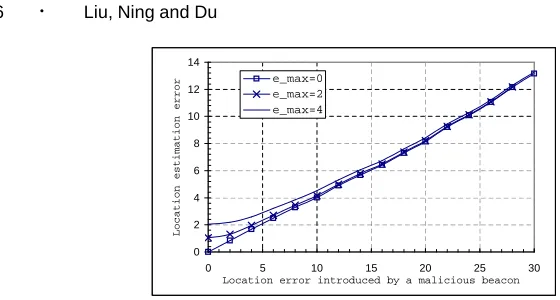
Fig. 2. Location estimation error. Unit of measurement forxandyaxes: meter
to use the “inconsistency” among the location references to identify the malicious ones, and discard them before finally estimating the locations at sensor nodes.
In this paper, we assume a sensor node uses a MMSE-based method (e.g., [Savvides et al. 2001; Savvides et al. 2002; Niculescu and Nath 2003a; Nasipuri and Li 2002; Do-herty et al. 2001; Niculescu and Nath 2003b]) to estimate its own location. Thus, most current range-based localization methods can be used with this technique. To harness this observation, we first estimate the sensor’s location with the MMSE-based method and then assess if the estimated location could be derived from a set of consistent location refer-ences. If yes, we accept the estimation result; otherwise, we identify and remove the most “inconsistent” location reference, and repeat the above process. This process may continue until we find a set of consistent location references or it is not possible to find such a set.
3.1 Checking the Consistency of Location References
We use the mean square errorς2 of the distance measurements based on the estimated
location as an indicator of the degree of inconsistency, since all the MMSE-based methods estimate a sensor node’s location by (approximately) minimizing this mean square error. Other indicators are possible but need further investigation.
DEFINITION 1. Given a set of location referencesL = {hx1, y1, δ1i,hx2, y2, δ2i, ...,
hxm, ym, δmi}and a location(˜x0,˜y0)estimated based onL, the mean square error of this
location estimation is
ς2=
m
X
i=1 (δi−
p
(˜x0−xi)2+ (˜y0−yi)2)2
m .
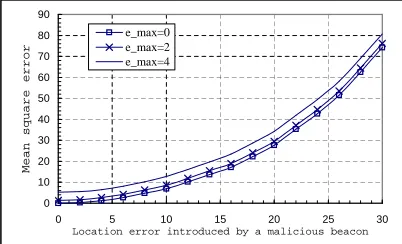
Intuitively, the more inconsistent a set of location references is, the greater the corre-sponding mean square error should be. To gain further understanding, we performed an experiment through simulation with the MMSE-based method in [Savvides et al. 2001].
We assume the distance measurement error is uniformly distributed between−emaxand
emax. We used 9 honest beacon nodes and 1 malicious beacon node evenly deployed in a
30m×30mfield. The node that estimates location is positioned at the center of the field. The malicious beacon node always declares a false location that isxmeters away from its real location, wherexis a parameter in our experiment.
0 10 20 30 40 50 60 70 80 90
0 5 10 15 20 25 30
Location error introduced by a malicious beacon
Mean square error
e_max=0 e_max=2 e_max=4
Fig. 3. Mean square errorς2
. Unit of measurement forx-axis: meter
As these figures show, if a malicious beacon node increases the location estimation error by introducing greater errors, it also increases the mean square errorς2at the same time. This further demonstrates that the mean square errorς2is potentially a good indicator of inconsistent location references.
In this paper, we choose a simple, threshold-based method to determine if a set of loca-tion references is consistent. Specifically, a set of localoca-tion referencesL ={hx1, y1, δ1i, hx2, y2, δ2i, ..., hxm, ym, δmi}obtained at a sensor node isτ-consistent w.r.t. a
MMSE-based method if the method gives an estimated location(˜x0,y0˜ )such that the mean square error of this location estimation
ς2=
m
X
i=1 (δi−
p
(˜x0−xi)2+ (˜y0−yi)2)2
m ≤τ
2.
3.2 Determining Thresholdτ
The determination of thresholdτdepends on the measurement error model, which is
as-sumed to be available for us to perform simulation off-line and determine an appropriate
τ. The threshold is stored on each sensor node. Usually, the movement of sensor nodes
(beacon or non-beacon nodes) does not have significant impact on this threshold, since the measurement error model will not change significantly in most cases. However, when the error model changes frequently and significantly, the performance of our techniques may be affected. In this paper, we assume the measurement error model will not change.
Note that the malicious beacon signals usually increase the variance of estimation. Thus, having a lower bound (e.g., Cramer-Rao bound) is not enough for us to filter malicious beacon signals. In fact, the upper bound or the distribution of the mean square error are more desirable. In this paper, we study the distribution of the mean square errorς2when there are no malicious attacks, and use this information to help determine the thresholdτ. Since there is no other error besides the distance measurement error, a benign location referencehx, y, δiobtained by a sensor node at(x0, y0)must satisfy:
|δ−p(x−x0)2+ (y−y0)2| ≤ǫ,
whereǫis the maximum distance measurement error.
square errorς2using the real location as the estimated location, and compare it with the distribution obtained through simulation when there are location estimation errors.
The measurement error of a benign location referencehxi, yi, δiican be computed as
ei=δi−
p
(x0−xi)2+ (y0−yi)2, where(x0, y0)is the real location of the sensor node.
Assuming the measurement errors introduced by different benign location references are independent, we can get the distribution of the mean square error through the following Lemma.
LEMMA 1. Let{e1, ..., em} be a set of independent random variables, andµi,σ2i be
the mean and the variance ofe2
i, respectively. If the estimated location of a sensor node is
its real location, the probability distribution ofς2is
lim
m→∞F[ς
2
≤ς02] = Φ( mς2
0 −µ
′
σ′ ),
whereµ′
=Pm
i=1µi,σ′ =pPim=0σi2, andΦ(x)is the probability of a standard normal
random variable being less thanx.
PROOF. Obviously, the mean square error can be computed byς2 = Pm
i=1
e2 i
m. Thus,
the cumulative distribution function can be calculated by
F(ς2≤ς02) =F(
m
X
i=1
e2i ≤mς02).
Since{e21, e22,· · ·, e2m}are independent, according to the central limit theorem, we have
lim
m→∞P(
Sm−µ′
σ′ ≤x) = Φ(x),
whereSm=Pmi=0(e2i). Thus, we have
limm→∞F(ς2≤ς02) = limm→∞F(Sm≤mς02)
= limm→∞P(S
m−µ′
σ′ ≤
mς2 0−µ′
σ′ )
= Φ(mς
2 0−µ′
σ′ )
Lemma 1 describes the probability distribution ofς2based on a sensor’s real location.
Though it is different from the probability distribution ofς2based on a sensor’s estimated
location, it can be used to approximate such distribution in most cases.
Let us further assume a simple model for measurement errors, where the measurement error is evenly distributed between−ǫandǫ. Then the mean and the variance foreiare 0
andǫ32, respectively, and the mean and the variance for anye2i are ǫ32 and445ǫ4, respectively. Letc= ς0
ǫ, we have
F(ς2≤(c×ǫ)2) = Φ( √
5m(3c2−1)
2 ).
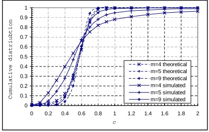
Figure 4 shows the probability distribution ofς2 derived from Lemma 1 and the
sim-ulated results using sensors’ estimated locations. We can see that when the number of location referencesmis large (e.g.,m= 9) the theoretical result derived from Lemma 1
0 0.1 0.2 0.3 0.4 0.5 0.6 0.7 0.8 0.9 1
0 0.2 0.4 0.6 0.8 1 1.2 1.4 1.6 1.8 2
c
Cumulative distriubtion
m=4 theoretical m=5 theoretical m=9 theoretical m=4 simulated m=5 simulated m=9 simulated
Fig. 4. Cumulative distribution functionF(ς2 ≤ς2
0). Letc= ς0
ǫ.
are observable differences between the theoretical results and the simulation. The reasons are twofold. First, our theoretical analysis is based on the central limit theorem, which is
only an approximation of the distribution whenmis a large number. Second, we used the
MMSE-based method proposed in [Savvides et al. 2001] in the simulation, which estimates a node’s location by only approximately minimizing the mean square error. (Otherwise, the value ofς2for benign location references should never exceedǫ2.)
Figure 4 gives three hints about the choice of the thresholdτ. First, when there are enough number of benign location references, a threshold less than the maximum
mea-surement error is enough. For example, whenm = 9,τ = 0.8ǫcan guarantee the nine
benign location references are considered consistent with high probability. Besides, a large threshold may lead to the failure to filter out malicious location references. Second, when
mis small (e.g. 4), the cumulative probability becomes flatter and flatter whenc >0.8.
This means that setting a large thresholdτ for smallmmay not help much to guarantee
the consistency test for benign location references; instead, it may give an attacker high chance to survive the detection. Third, the threshold cannot be too small; otherwise, a set of benign location references has high probability to be determined as a non-consistent reference set.
Based on the above observations, we propose to choose the value forτ with a hybrid
method. Specifically, when the number of location references is large (e.g., more than
8), we determine the value ofτ based on Lemma 1. Specifically, we choose a value of
τ corresponding to a high cumulative probability (e.g., 0.9). When the number location
references is small, we perform simulation to derive the actual distribution of the mean square error, and then determine the value ofτ accordingly. Since there are only a small number of simulations to run, we believe this approach is practical.
3.3 Identifying the Largest Consistent Set
Since the MMSE-based methods can deal with measurement errors better if there are more benign location references, we should keep as many benign location references as possi-ble when the malicious ones are removed. This implies we should get the largest set of consistent location references.
3.3.1 Brute-force Algorithm. Given a setLofnlocation references and a threshold
check all subsets ofLwithilocation references aboutτ-consistency, whereistarts from
nand drops until a subset ofLis found to beτ-consistent or it is not possible to find such a set. Thus, if the largest set of consistent location references consists ofmelements, a
sensor node has to use the MMSE method at least1 + n
m+1
+· · ·+ n n
times to find out
the right one. Ifn= 10andm = 5, a node needs to perform the MMSE method for at
least 387 times. It is certainly not desirable to do such expensive operations on resource constrained sensor nodes.
3.3.2 Greedy Algorithm. To reduce the computation on sensor nodes, we may use a
greedy algorithm, which is simple but suboptimal. This greedy algorithm works in rounds. It starts with the set of all location references in the first round. In each round, it first verifies if the current set of location references isτ-consistent. If yes, the algorithm outputs the estimated location and stops. Optionally, it may also output the set of location references. Otherwise, it considers all subsets of location references with one fewer location reference, and chooses the subset with the least mean square error as the input to the next round. This algorithm continues until it finds a set ofτ-consistent location references or when it is not possible to find such a set (i.e., there are only 3 remaining location references).
The greedy algorithm significantly reduces the computational overhead in sensor nodes. To continue the earlier example, a sensor node only needs to perform MMSE operations for about 50 times (instead of 387 times) using this algorithm. In general, a sensor node needs to use a MMSE-based method for at most1 +n+ (n−1)+· · ·+ 4 = 1 +(n−3)(n+4)
2
times.
However, as we mentioned, the greedy algorithm cannot guarantee that it can always identify the largest consistent set. It is possible that benign location references are re-moved. In out earlier version of this paper [Liu et al. 2005a], we note that this generates a big impact on the accuracy of location estimation – especially when there are multiple malicious location references. To deal with this problem, we develop an enhanced greedy algorithm in the following. The new algorithm is based on an efficient approach to identi-fying the most suspicious location reference from a set of location references.
3.3.3 Enhanced Greedy Algorithm. In the previous discussion, we only consider the
consistency of 3 or more location references. A further investigation also reveals that two benign location references are usually “consistent” with each other in the sense that there exists at least one location in the deployment field on which both location references agree. Hence, when the majority of location references are benign, we can usually find many location references that are consistent with a benign location reference. In addition, when a malicious location reference tries to create a larger location error, the number of location references that are consistent with the malicious one will decrease quickly.
According to the above discussion, for each location reference, we simply count the number of location references that are consistent with this location reference. We call this number the degree of consistency and use it to rank the suspiciousness of the location references received at a particular non-beacon node. The smaller the degree is, the more likely that the corresponding location reference is malicious.
error. For the sake of presentation, we refer to such a ring a candidate ring (centered)
at location(x, y). The non-beacon node then check whether the candidate rings of two location references overlap each other. If yes, they are consistent; otherwise, they are not consistent.
The algorithm to check whether the candidate rings of two location referencesa =
hxa, ya, δai andb = hxb, yb, δbi overlap can be done efficiently in the following way.
Letdab denote the distance between(xa, ya)and(xb, yb). Letrmax(x)andrmin(x)
denote the outer radius and the inner radius of the candidate ring of location reference
xrespectively. We can easily figure out that the candidate rings of location referencesa
andb will not overlap when either of the following three conditions is true: (1)dab >
rmax(a) +rmax(b), (2)dab+rmax(a)< rmin(b)and (3)dab+rmax(b)< rmin(a).
Similar to the greedy algorithm, the enhanced algorithm to identify the largest consis-tent set starts with the set of all location references in the first round. In each round, it verifies whether the current set of location references isτ-consistent. If yes, the algorithm outputs the estimated location and stops. Optionally, it may also output the set of location references. If not, it removes the location reference corresponding to the smallest degree and use the remaining location references as the input to the next round. This algorithm continues until it finds a set ofτ-consistent location references or when it is not possible to find such a set (i.e., there are only 3 remaining location references).
The enhanced algorithm not only improves the accuracy of location estimation in the presence of malicious attacks, but also reduces the computation overhead significantly since it can identify the most suspicious location reference efficiently and effectively. To continue the earlier example, a non-beacon node only needs to perform MMSE operations for 5 times. In general, a non-beacon node needs to use a MMSE-based method for at most
n−3times.
4. VOTING-BASED LOCATION ESTIMATION
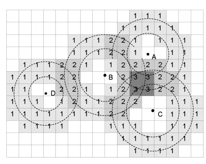
In this approach, we have each location reference “vote” on the locations at which the node of concern may reside. To facilitate the voting process, we quantize the target field into a grid of cells, and have each sensor node determine how likely it is in each cell based on each location reference. We then select the cell(s) with the highest vote and use the “center” of the cell(s) as the estimated location. To deal with the resource constraints on sensor nodes, we further develop an iterative refinement scheme to reduce the storage overhead, improve the accuracy of estimation, and make the voting scheme efficient on resource constrained sensor nodes.
4.1 The Basic Scheme
After collecting a set of location references, a sensor node should determine the target field. The node does so by first identifying the minimum rectangle that covers all the locations declared in the location references, and then extending this rectangle byRb, whereRbis
the maximum transmission range of a beacon signal. This extended rectangle forms the target field, which contains all possible locations for the sensor node. The sensor node then divides this rectangle intoM small squares (cells) with the same side lengthL, as illustrated in Figure 5. (The node may further extend the target field to have square cells.) The node then keeps a voting state variable for each cell, initially set to 0.
Fig. 5. The voting-based location estimation
candidate ring at A, which is derived from the location reference with the declared location at A.
For each location referencehx, y, δi, the sensor node identifies the cells that overlap with the corresponding candidate ring, and increments the voting variables for these cells by 1. After the node processes all the location references, it chooses the cell(s) with the highest vote, and uses its (their) geometric centroid as the estimated location of the sensor node.
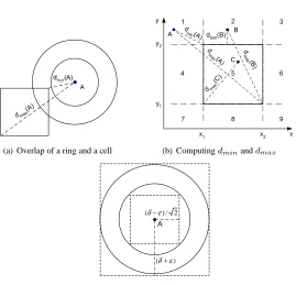
4.2 Overlap of Candidate Rings and Cells
A critical problem in the voting-based approach is to determine if a candidate ring overlaps with a cell. We discuss how to determine this efficiently below.
Suppose we need to check if the candidate ring at A overlaps with the cell shown in
Figure 6(a). Let dmin(A) anddmax(A)denote the minimum and maximum distances
from a point in the cell to point A, respectively. We can see that the candidate ring does not overlap with the cell only whendmin(A)> roordmax(A)< ri, whereri = max{0, δ−
ǫ}andro=δ+ǫare the inner and the outer radius of the candidate ring, respectively.
To computedminanddmax, we divide the target field into 9 regions based on the cell,
as shown in Figure 6(b). It is easy to see that given the center of any candidate ring, we can determine the region in which it falls with at most 6 comparisons between the coordinates of the center and those of the corners of the cell. When the center of a candidate ring is in region 1 (e.g., point A in Figure 6(b)), it can be shown that the closest point in the cell to A is the upper left corner, and the farthest point in the cell from A is the lower right corner. Thus,dmin(A)anddmax(A)can be calculated accordingly. These two distances can be
computed similarly when the center of a candidate ring falls into regions 3, 7, and 9. Consider point B in region 2. Assume the coordinate of point B is(xB, yB). We can see
thatdmin(B) =yB−y2. Computingdmax(B)is a little more complex. We first need to
check ifxB−x1> x2−xB. If yes, the farthest point in the cell from B must be the lower
left corner of the cell. Otherwise, the farthest point in the cell from B should be the lower right corner of the cell. Thus, we have
dmax(B) =
p
(max{xB−x1, x2−xB})2+ (yB−y1)2.
dmin(A)
d m ax( A )
A
(a) Overlap of a ring and a cell
x y
x1 x2
y1
y2
1 2 3
4 5 6
7 8 9
dm i n (A)
dm
ax(A)
dmin(B)
d
m
a x(B )
dma x ( C)
A B
C
(b) Computingdminanddmax
A 2 / )
(δ−ε
)
(δ+ε
(c) Limiting the examinations of cells
Fig. 6. Determine whether a ring overlaps with a cell
into regions 4, 6, and 8.
Consider a point C in region 5. Obviously,dmin(C) = 0since point C itself is in the
cell. Assume the coordinate of point C is(xc, yc). The farthest point in the cell from C
must be one of its corners. Similarly to the above case for point B, we may check which point is farther away from C by checkingxc−x1> x2−xcandyc−y1> y2−yc. As a
result, we get
dmax(C) =
p
(max{xc−x1, x2−xc})2+ (max{tc−y1, y2−yc})2.
Based on the above discussion, we can determine if a cell and a candidate ring overlap with at most 10 comparisons and a few arithmetic operations. To prove the correctness of the above approach only involves elementary geometry, and thus is omitted.
For a given candidate ring, a sensor node does not have to check all the cells for which it maintains voting states. As shown in Figure 6(c), with simple computation, the node can get the outer bounding box centered at A with side length2(δ+ǫ). The node only needs to consider the cells that intersect with or fall inside this box. Moreover, the node can get the inside bounding box with simple computation, which is centered at A with side length √
2(δ−ǫ), and all the cells that fall into this box need not be checked.
4.3 Iterative Refinement
storage is required. Second, the value ofM (orL) determines the precision of location estimation. The largerM is, the smaller each cell will be. As a result, a sensor node can determine its location more precisely based on the overlap of the cells and the candidate rings.
However, due to the resource constraints on sensor nodes, the granularity of the partition is usually limited by the memory available for the voting state variables on the nodes. This puts a hard limit on the accuracy of location estimation. To address this problem, we propose an iterative refinement of the above basic algorithm to achieve fine accuracy with reduced storage overhead.
In this version, the number of cellsM is chosen according to the memory constraint in a sensor node. After the first round of the algorithm, the node may find one or more cells having the largest vote. To improve the accuracy of location estimation, the sensor node then identifies the smallest rectangle that contains all the cells having the largest vote, and performs the voting process again. For example, in Figure 5, the same algorithm will be performed in a rectangle which exactly includes the 4 cells having 3 votes. Note that in a later iteration of the basic voting-based algorithm, a location reference does not have to be used if it does not contribute to any of the cells with the highest vote in the current iteration. Due to a smaller rectangle to quantize in a later iteration, the size of cells can be reduced, resulting in a higher precision. Moreover, a malicious location reference will most likely be discarded, since its candidate ring usually does not overlap with those derived from benign location references. For example, in Figure 5, the candidate ring centered at point D will not be used in the second iteration.
The iterative refinement process should terminate when a desired precision is reached or the estimation cannot be refined. The former condition can be tested by checking if the side lengthLof each cell is less than a predefined thresholdS, while the latter condition
can be determined by checking whetherLremains the same in two consecutive iterations.
The algorithm then stops and outputs the estimated location obtained in the last iteration. It is easy to see that the algorithm will fall into either of these two cases, and thus will alway terminate. In practice, we may set the desired precision to 0 in order to get the best precision.
5. SECURITY ANALYSIS
Both proposed techniques can usually remove the effect of the malicious location refer-ences from the final location estimation when there are more benign location referrefer-ences than the malicious ones. Theorem 1 shows that when the majority of location references are benign, the location estimation error of the attack-resistant MMSE is bounded if we can successfully identify the largest consistent set. Hence, to defeat the attack-resistant MMSE approach, the attacker has to distribute to a victim node more malicious location references than the benign ones, and control the declared locations and the physical fea-tures (e.g., signal strength) of beacon signals so that the malicious location references are considered consistent.
LEMMA 2. Assume there arembenign location references andnmalicious location
references in aτ-consistent set. The location estimation error from this set of location
ref-erences using MMSE is no more than2R+qm+n
m τ, whereRis the radio communication
PROOF. LetO = (x0, y0)denote the real location of the non-beacon node andO′ = (x′
0, y
′
0)denote the estimated location of the non-beacon node based on all location
ref-erences (including the malicious ones). Let|AB|denote the distance betweenAandB. Thus, the location estimation error can be represented by|OO′
|. Let{L1,· · ·, Lm}denote
the set of benign location references and{Lm+1,· · ·, Lm+n}denote the set of malicious
location references.
Consider a particular benign location referencesLi =hxi, yi, δii. Since the
communi-cation range of sensor nodes isR, we have|OLi| ≤R. In addition,ei =δi− |O′Li|and
δi≤R. Thus, we have
|OO′
| ≤ |OLi|+|LiO
′
| ≤R+δi−ei≤2R−ei.
There are two different cases: ei ≥0orei <0. Whenei ≥0, we have|OO′| ≤2R.
When ei < 0, we have |OO′| −2R ≤ −ei. Assume |OO′| ≥ 2R, we have e2i ≥
(|OO′
| −2R)2. Since{L1,· · ·, L
m+n}isτ-consistent, we havePim=1+ne2i ≤(m+n)τ2.
Therefore,
m(|OO′
| −2R)2≤
m
X
i=1 e2i ≤
m+n
X
i=1
e2i ≤(m+n)τ2.
Hence, we have(|OO′
| −2R)2≤ (m+n)τ2
m . It implies
|OO′
| ≤2R+
r
m+n m τ.
According to the above analysis, we can conclude that the statement in Lemma 2 is true.
THEOREM 1. Assume a non-beacon node receivesmbenign location references andn
malicious loccation references, wherem > n. The location estimation error at this non-beacon node using the attack-resistant MMSE scheme with the brute-force algorithm is no more than2R+q m
m−nτif the thresholdτis set greater than the maximum distance error
ǫ, whereRis the radio communication range of a sensor node.
PROOF. It is easy to know that the set of mbenign location references is always τ -consistent ifτ ≥ǫ. Thus, there are at leastmlocation references in the largest consistent set. Assume there areklocation references in the largest consistent set, wherek ≥ m. According to Lemma 2, we have
|OO′
| ≤2R+
r
k
k−nτ≤2R+
r
m m−nτ.
Similarly, theorem 2 shows that when the majority of location references are benign, the location estimation error of the voting-based scheme is bounded. Hence, to defeat the voting-based approach, the attacker needs similar efforts so that the cell containing the attacker’s choice gets more votes than those containing the sensor’s real location.
THEOREM 2. When the majority of location references at a non-beacon node are
PROOF. Assume the real location of the sensor node isO = (x0, y0)and the estimated
location of the sensor node using the voting-based scheme isO′ = (x′
0, y
′
0).
Since the candidate ring of a benign location reference always covers the real locationO
of the sensor node, the number of votes in the cell that containsOis at leastm. Thus, the number of votes in the cell that containsO′
is at leastm. Since the number of votes coming from the malicious location references is at most n, we know that there is at least one benign location reference whose candidate ring covers the cell that containsO′
. Assume one of such benign location referecnes isLi=hxi, yi, δii, we have
|LiO
′
| ≤R+√2L,
whereLis the side length of a cell. Therefore, we have
|OO′
| ≤ |OLi|+|LiO
′
| ≤2R+√2L.
An attacker has two ways to satisfy the above conditions (in order to defeat our tech-niques). First, the attacker may compromise beacon nodes and then generate malicious beacon signals. Since all beacon packets are authenticated, and a sensor node uses at most one location reference derived from the beacon signals sent by each beacon node, the at-tacker needs to compromise more beacon nodes than the benign beacon nodes from which a target sensor node may receive beacon signals, besides carefully crafting the forged bea-con signals.
Second, the attacker may launch wormhole attacks [Hu et al. 2003] (or replay attacks) to tunnel benign beacon signals from one area to another. In this case, the attacker does not have to compromise any beacon node, though he/she has to coordinate the wormhole attacks. This paper does not provide techniques to address wormhole attacks. However, our methods can still tolerate wormhole attacks to a certain degree as long as the number of malicious location references at a sensor node is less than the number of benign location references. On the other hand, we may also use some of existing wormhole detection methods (e.g., packet leashes [Hu et al. 2003], directional antennae [Hu and Evans 2003b]) to make it more difficult for an attacker to introduce many malicious location references to a sensor node by launching wormhole attacks.
Our techniques certainly have a limit. In an extreme case, if all the beacon nodes are compromised, our techniques will fail. However, the proposed techniques offer a graceful performance degradation as more malicious location references are introduced. In con-trast, an attacker may introduce arbitrary location error with a single malicious location reference in the previous schemes. To further improve the security of location discovery, other complementary mechanisms (e.g., detection of malicious beacon nodes) should be used.
6. SIMULATION EVALUATION
This section presents the simulation results for both proposed schemes. The evaluation focuses on the performance under different configurations and the improvement on the accuracy of location estimation in hostile environments.
Three attack scenarios are considered. The first scenario considers a single malicious
real location. (An attacker may also modify the distance componentδin a location ref-erence, which will generate a similar impact.) In the second scenario, there are multiple non-colluding malicious location references, and each of them independently declares a
wrong location that isemeters away from the beacon node’s real location. In the third
scenario, multiple colluding malicious location references are considered. In this case, the malicious location references declare false locations by coordinating with each other to create a virtual locationemeters away from the sensor’s real location. Thus, the malicious location references may appear to be consistent to a victim node.
In all simulations, a set of benign beacon nodes and a few malicious beacon nodes are evenly deployed in a30m×30mtarget field. The non-beacon sensor node is located at the center of this target field. We assume the maximum transmission range of beacon signals is
Rb = 22m, so that the non-beacon node can receive the beacon signal from every beacon
node located in the target field. We assume the entire deployment field is much larger than this target field so that an attacker can create a very large location estimation error inside the deployment field. Each malicious beacon node declares a false location according to the three attack scenarios discussed above. We assume a simple distance measurement error model. That is, the distance measurement error is uniformly distributed between−ǫ
andǫ, where the maximum distance measurement errorǫis set toǫ= 4m.
6.1 Evaluation of Attack-Resistant MMSE
In the simulation, we use the MMSE-based method proposed in [Savvides et al. 2001], which we call the basic MMSE method, to perform the basic location estimation. Our attack-resistant MMSE method is then implemented on the basis of this method, as dis-cussed in Section 3. We setτ = 0.8ǫaccording to Figure 4, which guarantees9benign location references are considered consistent with probability of0.999.
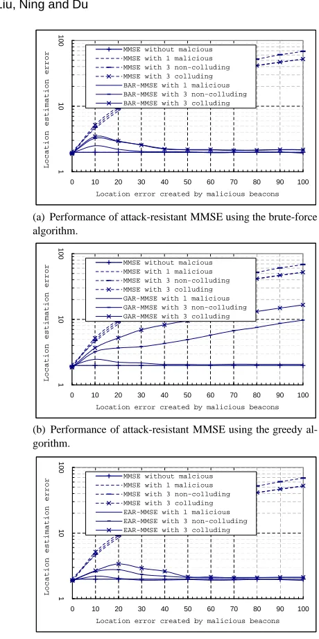
Figure 7(a) shows the performance of the attack-resistant MMSE method when the brute-force algorithm is used to identify the largest consistent set. We can see that our technique can significantly reduce the location estimation error when there are malicious location references. The figure also indicates that when the malicious location references create large location errors, they are always removed from the final location estimation at a non-beacon node.
Figure 7(b) shows the performance of the attack-resistant MMSE method when the greedy algorithm is used to identify the largest consistent set. From the figure, we can see that the technique can significantly reduce the location estimation error when there is only one malicious location reference. However, the performance degrades quickly when there are multiple malicious location references. This is because multiple malicious lo-cation references, especially when they collude together, make the filtering of malicious location references more difficult. It is very possible that benign location references being identified as malicious and being removed. Hence, we know that the greedy algorithm can-not effectively identify the largest consistent set when there are more than one malicious location references.
1
1
0
0
0 10 20 30 40 50 60 70 80 90 100
Location error created by malicious beacons
L o c a t i o n e s t i m a t i o n e r r o
r MMSE without malcious
MMSE with 1 malicious MMSE with 3 non-colluding MMSE with 3 colluding BAR-MMSE with 1 malicious BAR-MMSE with 3 non-colluding BAR-MMSE with 3 colluding
(a) Performance of attack-resistant MMSE using the brute-force algorithm. 1 1 0 1 0 0
0 10 20 30 40 50 60 70 80 90 100
Location error created by malicious beacons
L o c a t i o n e s t i m a t i o n e r r o
r MMSE without malcious
MMSE with 1 malicious MMSE with 3 non-colluding MMSE with 3 colluding GAR-MMSE with 1 malicious GAR-MMSE with 3 non-colluding GAR-MMSE with 3 colluding
(b) Performance of attack-resistant MMSE using the greedy al-gorithm. 1 1 0 1 0 0
0 10 20 30 40 50 60 70 80 90 100
Location error created by malicious beacons
L o c a t i o n e s t i m a t i o n e r r o
r MMSE without malcious
MMSE with 1 malicious MMSE with 3 non-colluding MMSE with 3 colluding EAR-MMSE with 1 malicious EAR-MMSE with 3 non-colluding EAR-MMSE with 3 colluding
(c) Performance of attack-resistant MMSE using the enhanced greedy algorithm
Fig. 7. τ= 0.8ǫ. Unit of measurement forxandyaxes: meter
enhanced greedy algorithm is used in the attack-resistant MMSE method.
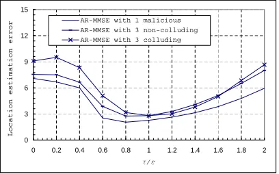
From 7(c), we note that the malicious location references can generate big impact when the location errors created by them are around20m. Therefore, we assume that malicious location references introduce20m location errors and evaluate the effect of thresholdτ
0 3 6 9 12 15
0 0.2 0.4 0.6 0.8 1 1.2 1.4 1.6 1.8 2
/
L
o
c
a
t
i
o
n
e
s
t
i
m
a
t
i
o
n
e
r
r
o
r AR-MMSE with 1 malicious
AR-MMSE with 3 non-colluding AR-MMSE with 3 colluding
Fig. 8. Performance of Attack-resistant MMSE under different thresholdτ. Assume each malicious location reference introduces20m location error.
thresholdτcannot be set too large or too small since it will either fail to remove malicious location references or remove a large number of benign location references. This result is consistent with our analysis in Section 3.2.
6.2 Evaluation of Voting-Based Scheme
0 0.5 1 1.5 2 2.5 3 3.5
0 25 50 75 100 125 150 175 200
The granularity of partition (M)
Location estimation error
e=0
e=10
e=50
Fig. 9. Performance for differentM(e: error introduced by a malicious location reference)
We first study the impact of parameterM on the voting-based method. Figure 9 shows
the performance of the voting-based scheme with different values ofM when there is only one malicious location reference. We can see that the location estimation error initially
decreases whenM increases, but then does not decrease much whenM is greater than
100. Moreover, the parameterM also has implications in computational cost. Since the
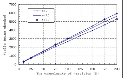
voting-based method is finally reduced to checking whether a candidate ring derived from a location reference overlaps with the cells in the grid, we use the number of cells being ex-amined as an indicator of the computational cost. Figure 10 shows the computational costs of the voting-based method for different values ofM when there is one malicious location reference. As this figure shows, the computational cost increases almost linearly with the
value ofM. When there are no or more malicious location references, the computational
implies 100 Bytes memory for the voting variables, in the later simulations to trade-off the accuracy with the storage and computation overhead.
0 1000 2000 3000 4000 5000 6000 7000
0 25 50 75 100 125 150 175 200
The granularity of partition (M)
#cells being checked
e=0
e=10
e=50
Fig. 10. Computational cost for differentM(e: error introduced by a malicious location reference)
Next, we study the performance of the voting-based scheme under malicious attacks. In the simulation, we also setS= 0to get the minimum location estimation error achievable by this method. Figure 11 compares the accuracy of the basic MMSE method and our voting-based scheme under different types of attacks. We can clearly see that the accuracy of location estimation is improved significantly in our scheme. In addition, unlike the attack-resistant MMSE scheme, the voting-based scheme can tolerate multiple (colluding or non-colluding) malicious location references more effectively.
1 10 100
0 10 20 30 40 50 60 70 80 90 100
Location error introduced by malicious beacons
L
o
c
a
t
i
o
n
e
s
t
i
m
a
t
i
o
n
e
r
r
o
r MMSE without malicious
MMSE with 1 malicious MMSE with 3 non-colluding MMSE with 3 colluding Voting with 1 malicious Voting with 3 non-colluding Voting with 3 colluding
Fig. 11. Performance of the voting-based scheme (M = 100, S = 0). Unit of measurement forxandyaxes: meter
also note that the performance of voting-based scheme under attacks is usually better than the performance of MMSE scheme without attacks. This is because we used the MMSE-based method in [Savvides et al. 2001] in the simulation, which estimates a node’s location by only approximately minimizing the mean square error.
Now let us compare the attack-resistant MMSE and the voting-based methods. Based on the earlier results, we choose thresholdτ = 0.8ǫfor the attack-resistant MMSE, and set
M = 100andS = 0for the voting-based scheme. Figure 12 shows that the voting-based
scheme performs slightly better than the attack-resistant MMSE scheme in terms of the location estimation accuracy when there are malicious location references.
1
1
0
0 10 20 30 40 50 60 70 80 90 100
Location error created by malicious beacon
L
o
c
a
t
i
o
n
e
s
t
i
m
a
t
i
o
n
e
r
r
o
r EAR-MMSE with 1 maliciousEAR-MMSE with 3 non-colluding
EAR-MMSE with 3 colluding Voting with 1 malicious Voting with 3 non-colluding Voting with 3 colluding
Fig. 12. Comparison between the attack-resistant MMSE and the voting-based scheme. Unit of measurement: meter
7. IMPLEMENTATION AND FIELD EXPERIMENTS
We have implemented both schemes on TinyOS [Hill et al. 2000], an operating system for networked sensors. These implementations are targeted at MICA2 motes [Crossbow Technology Inc. ] running TinyOS. The attack-resistant MMSE is implemented based on the basic MMSE method proposed in [Savvides et al. 2001]. However, our implementation of the basic MMSE method is simplified by only using the location coordinates (without the ultrasound propagation speed, which is not necessary in our study).
Scheme ROM (bytes) RAM (bytes)
MMSE 2034 286
EAR-MMSE 3738 434
Voting-Based 4488 174
Table I. Code size (assume 12 location references;M= 100)
Table I gives the code size (ROM and RAM) for these implementations on MICA2 platform. Table I is obtained by assuming at most 12 location references. More location references will increase the RAM size of the program, but the increased RAM is only required to save the additional location references.
0.001 0.01 0.1 1 10
4 6 8 10 12 14 16 18 20 22 24 26
Number of location references
Time (sec)
MMSE
EAR-MMSE
Voting
(a) A single malicious location reference
0.001 0.01 0.1 1 10
0 1 2 3 4 5
Number of malicious location references
Time (sec)
MMSE
EAR-MMSE
Voting
(b) A total of 12 location references
Fig. 13. Average execution time on MICA2 motes (ǫ = 4m, τ = 0.8ǫ,M = 100and
S= 0)
by counting the numbers of CPU clock cycles spent on location estimation. The location references used in the experiment are generated from the simulation in Section 6. We can see that the basic MMSE method has the least execution time. The attack-resistant MMSE scheme has less computational cost than the voting-based scheme. The number of malicious location references does not affect the computational overheads of the basic MMSE method and the voting-based method but does affect the computational overhead of the attack-resistant MMSE method. From Table I and Figure 13, we conclude that our proposed techniques are practical for the current generation of sensor networks in terms of the storage and the computation overheads, especially when the locations of sensor nodes do not change frequently.
To further study the feasibility of our techniques, we performed an outdoor field
exper-iment. In this experiment, eight MICA2 motes were deployed in a10×10target field,
where each unit of distance is 4 feet, as shown in Figure 14. The sensor node with ID 0 is configured as a non-beacon node, which is located at the center of the field. All the other sensor nodes are configured as beacon nodes.
We considered three attack scenarios in this experiment. In the first scenario, beacon
node 1 is configured as a malicious beacon node that always declares a locatione feet
0
0 1 2 3 4 5 6 7 8 9 10
1
2
3
4
5
6
7
8
9
10
Sensor ID=0 Beacon ID=1
(1,3) Beacon
ID=2 (2,6)
Beacon ID=3 (4,4)
Beacon ID=4 (4,9)
Beacon ID=5 (9,5) Beacon
ID=6
(7,1) Beacon
ID=7 (8,8)
Fig. 14. Target area of field experiment.
scenario, beacon nodes1,2and3are configured as malicious beacon nodes. Each of these three nodes declares a locatione feet away from its real location in the directions away from the non-beacon node. In the third scenario, three malicious beacon nodes1,2, and 3 work together to create a virtual location. Each of these three nodes declares a false location by increasing its horizontal coordinate byefeet. This actually creates a virtual location in the horizontal axisefeet away from the non-beacon node’s real location. This is illustrated in Figure 14 by the horizontal arrow starting from the non-beacon node.
To measure the distance (δ) between sensor nodes, we use a simple RSSI based
tech-nique. Note that the Active Message protocol in TinyOS provides a reading in the strength field for the MICA2 platform. This value is returned in every received packet, and can be used to compute the signal strength. Thus, we performed an experiment before the actual field experiment to estimate the relationship between the values of this field and the dis-tance between two nodes. For each given disdis-tance, we computed the average of this values on20observations. We then built a table that contains distances and the corresponding av-erage readings. During the field experiments, when a sensor node receives20packets from a beacon node, it computes the average of the strength values, and estimates the distance with interpolation according to this table. For example, if the average readingv falls in between two adjacent points(vi, di)and(vi+1, di+1)in the table, the sensor computes the
distance
d=di+
(v−vi)×(di+1−di)
vi+1−vi
.
We setǫ to4 feet, which is the maximum distance measurement error observed in the
experiment.
Figure 15 shows the performance of the proposed methods and the basic MMSE method in the field experiment. For the first two attack scenarios, we can see that the proposed methods can tolerate malicious location references quite effectively. The performance in the third scenario is worse than the first two cases. The reason is that the non-beacon nodes
has only4benign location references, but3colluding location references. However, we
0 .1 1 1 0 0
0 20 40 60 80 100 120
Location error created by malicious beacons
L o c a t i o n e s t i m a t i o n e r r o r MMSE EAR-MMSE Voting
(a) A single malicious location reference
0 .1 1 1 0 0
0 20 40 60 80 100 120
Location error created by malicious beacons
L o c a t i o n e s t i m a t i o n e r r o r MMSE EAR-MMSE Voting
(b) 3 non-colluding malicious location reference
0 .1 1 1 0 1 0 0
0 20 40 60 80 100 120
Location error created by malicious beacons
L o c a t i o n e s t i m a t i o n e r r o r MMSE EAR-MMSE Voting
(c) 3 colluding malicious location reference
Fig. 15. Results of the field experiment. AssumeM = 100andS = 0for voting-based
scheme;τ= 0.8ǫ= 3.2feet for attack-resistant MMSE. Unit of measurement forxandy
axes: feet
the malicious attacks are above certain thresholds. Overall, the location estimation errors caused by malicious attacks are bounded when the proposed techniques are used, while the errors can be arbitrarily large when the basic MMSE method is used.
The field experiment further shows that our methods are efficient and effective in tol-erating malicious attacks. It also indicates that our methods are promising for the current generation of sensor networks.
8. RELATED WORK
and Nath 2003b]. None of these schemes will work properly when there are malicious attacks.
The location verification technique proposed in [Sastry et al. 2003] can verify the relative distance between a verifying node and a sensor node. It does not provide a solution to conduct secure location estimation at non-beacon nodes. In this paper, we provide efficient ways to estimate locations of sensor nodes securely. The location verification technique is complementary to our techniques since it can be used to enhance the security of distance measurement between two nodes.
A robust location detection is developed in [Ray et al. 2003]. However, it cannot be directly applied in sensor networks due to its high computation and storage overheads. A voting-based Cooperative Location Sensing (CLS) was proposed in [Fretzagias and Pa-padopouli 2004]. However, CLS is designed for powerful nodes (e.g., PDAs), while our scheme further uses iterative refinement to improve the performance with small storage overhead. Therefore, our technique can be implemented and executed efficiently on re-source constrained sensor nodes.
Similar to our attack-resistant location estimation techniques, the following two tech-niques are independently discovered to tolerate malicious attacks against location discov-ery in wireless sensor networks. A robust statistical methods that is similar to the attacker-resistant MMSE scheme is discovered in [Li et al. 2005] to achieve robustness through Least Median of Squares. A secure range-independent localization scheme (SeRLoc) that is similar to our voting-based scheme is discovered in [Lazos and Poovendran 2004] to protect location discovery with the help of sectored antennae at beacon nodes. Compared to these two studies, we provide more alternative ways to tolerate malicious attacks and also include the real implementation and field experiments in this paper.
SPINE [S.Capkun and Hubaux 2005] is developed to protect location discovery by using verifiable multilateration. However, the distance bounding techniques required for verifi-able multilateration may not be availverifi-able due to the difficulties to (1) deal with the external replay attacks in Ultrasound-based distance bounding and (2) achieve nanosecond process-ing and time measurements in Radio-based distance boundprocess-ing. ROPE [Lazos et al. 2005] is developed by integrating SerLoc and SPINE. However, it still requires nanosecond pro-cessing and time measurements that are not desirable for the current generation of sensor networks. Compared with these two studies, we provide techniques to tolerate malicious attacks without the above constraints. Moreover, our proposed techniques can be easily combined with most of existing localization techniques.
To further enhance the security of location discovery, a practical technique is developed to detect malicious beacon nodes that are providing malicious beacon signals [Du et al. 2005; Liu et al. 2005b]. This detection technique can be easily combined with our tech-niques. We consider it complementary to the techniques in this paper.
In addition to secure location discovery, location privacy becomes a more and more interesting topic recently. Several techniques are developed recently to protect the location privacy in sensor networks [Ozturk et al. 2004; Kamat et al. 2005].
Security in sensor networks has attracted a lot of attention in the past several years. To provide practical key management, researchers have developed key pre-distribution tech-niques [Eschenauer and Gligor 2002; Chan et al. 2003; Du et al. 2003]. To enable
broad-cast authentication, a protocol named µTESLA has been explored to adapt to resource
stud-ied in [Przydatek et al. 2003; Hu and Evans 2003a]. Attacks against routing protocols in sensor networks and possible counter measures were investigated in [Karlof and Wagner 2003]. The research in this paper addresses another fundamental security problem that has not drawn enough attention.
9. CONCLUSION AND FUTURE WORK
In this paper, we proposed an attack-resistant MMSE-based location estimation and a voting-based location estimation technique to deal with attacks in localization schemes. We have implemented the proposed techniques on MICA2 motes [Crossbow Technology Inc. ] running TinyOS [Hill et al. 2000], and evaluated them through both simulation and field experiments. Our experiences indicate that the proposed techniques are promising solutions for securing location discovery in wireless sensor networks.
Our future research is two-fold. First, we will study how to combine the proposed tech-niques with other protection mechanisms such as wormhole detection. Second, our simu-lations and experiments in this paper are conducted in small scales. It is very interesting to study the performance in a large scale.
Acknowledgment
The authors would like to thank the anonymous reviewers and Dr. Adrian Perrig for their valuable comments on the earlier version of this paper.
REFERENCES
AKYILDIZ, I., SU, W., SANKARASUBRAMANIAM, Y.,ANDCAYIRCI, E. 2002. Wireless sensor networks: A
survey. Computer Networks 38, 4, 393–422.
BULUSU, N., HEIDEMANN, J.,ANDESTRIN, D. 2000. GPS-less low cost outdoor localization for very small
devices. In IEEE Personal Communications Magazine. 28–34.
CHAN, H., PERRIG, A.,ANDSONG, D. 2003. Random key predistribution schemes for sensor networks. In IEEE Symposium on Research in Security and Privacy. 197–213.
CROSSBOW TECHNOLOGY INC. Wireless sensor networks. http://www.xbow.com/Products/
Wireless Sensor Networks.htm. Accessed in May 2005.
DOHERTY, L., PISTER, K. S.,ANDGHAOUI, L. E. 2001. Convex optimization methods for sensor node position
estimation. In Proceedings of INFOCOM’01.
DU, W., DENG, J., HAN, Y. S.,ANDVARSHNEY, P. 2003. A pairwise key pre-distribution scheme for wire-less sensor networks. In Proceedings of 10th ACM Conference on Computer and Communications Security (CCS’03). 42–51.
DU, W., FANG, L.,ANDNING, P. 2005. Lad: Localization anomaly detection for wireless sensor networks. In Proceedings of the 19th IEEE International Parallel & Distributed Processing Symposium (IPDPS ’05).
ESCHENAUER, L.ANDGLIGOR, V. D. 2002. A key-management scheme for distributed sensor networks. In
Proceedings of the 9th ACM Conference on Computer and Communications Security. 41–47.
FRETZAGIAS, C.ANDPAPADOPOULI, M. 2004. Cooperative location-sensing for wireless networks. In Second
IEEE International conference on Pervasive Computing and Communications.
GAY, D., LEVIS, P.,VONBEHREN, R., WELSH, M., BREWER, E.,ANDCULLER, D. 2003. The nesC language: A holistic approach to networked embedded systems. In Proceedings of Programming Language Design and Implementation (PLDI 2003).
HE, T., HUANG, C., BLUM, B. M., STANKOVIC, J. A.,ANDABDELZAHER, T. F. 2003. Range-free localization schemes in large scale sensor networks. In Proceedings of ACM MobiCom 2003.