Voronoi based face segmentation

6

VORONOI BASED FACE

SEGMENTATION

Abbas Cheddad

Dzulkifli Mohamad

1 INTRODUCTION

Image segmentation, decomposition of a gray level or color image into homogeneous tiles, is arguably the most important low-level vision task. Homogeneity is usually defined as similarity in pixel values. Segmentation is a fundamental process in digital image processing which has found extensive applications in areas such as content-based image retrieval, medical image processing, and remote sensing image processing. Its purpose is to extract labeled regions or boundaries for targeted objects for subsequent processing such as surface description and object recognition. A segmentation procedure usually consists of two steps. The first step is to choose a proper set of features which can identify the same-content regions and meanwhile differentiate different-content regions; the second step is to apply a segmentation method to the chosen features to achieve a segmentation map” (Deng H. and Clausi D., 2004). Segmentation is partition of an image I into a set of regions S satisfying:

„ Homogeneity predicate is satisfied by each region: ∀ Si,

P(Si) = true (3)

„ Union of adjacent regions does not satisfy it: P(Si ∪ Sj) =

false, i ≠ j, Si adjacent Sj (4)

Applications of image segmentation can be found in a wide variety of areas such as remote sensing, vehicle and robot navigation, medical imaging, surveillance, target identification and tracking, scene analysis, product inspection/ quality control, etc. Image segmentation remains a long standing problem in computer vision and it is found difficult and challenging for two main reasons (Tu Z. and Zhu S., 2002). The first challenge is the fundamental complexity of modeling a vast amount of visual data that appear in the image. The second challenge is the intrinsic ambiguity in image perception, especially when it concerns the so called unsupervised segmentation (e.g.: A decision whereby a region cut is not a trivial task).

In the process of information visualization, one usually will be in front of dot pattern rather than color images or gray level ones. The need for this is ultimately to have a system that can tolerate the situations where there is sensitivity of analysis to changes in lighting conditions, scale orientation of the camera, sensor characteristics, geometric distortion…etc. Such invariant and noise tolerant systems are proven to be useful in various industrial and military applications (Dowdall J. et al., 2003). Hence, extracting faces and facial features accurately and efficiently forms a wonderful problem. In addition to the above mentioned factors, the main problem is that facial features vary from individual to another in terms of shape and are highly deformable for one individual with multiple shots.

This makes choosing suitable points extremely critical for the performance of a given segmentation system.

The proposed method will accept a gray scaled image as an input, however the work is mostly on its binary version, which corresponds, to the simplest and yet one of the most useful image types. In general; a binary image is a representation of scenes with only two possible gray values for each pixel, typically 0 or 1. In many cases, an object shape boundary is usually used for pattern recognition and can be represented as follows:

f (x, y)=1,∀(x, y) ∈η (5)

f (x, y)=0,∀(x, y) ∉η (6)

Where

η denotes the region of the object in the image plane and x and y are the coordinates in the original image f. The binary image is useful in this study to extract easily labeled blobs and to feed them as input parameters to construct the Voronoi Diagram.

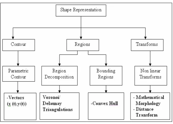
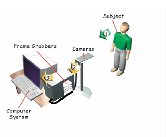
Figure 1 A block diagram for machine face recognition system

2 SYSTEM OVERVIEW

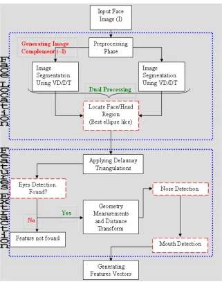
The proposed method is benefiting from Voronoi properties to detect and segment faces and the block diagram is shown in Figure 3. The first step in every machine vision task is the pre-processing phase, which includes (herein) and not limited to: Histogram Equalization, Mathematical Morphology, Median and low pass filtering. The dual processing is adopted to reduce as much as possible the mal effect of the intensive uneven illumination. The latter might introduce two problems, the first is creating holes in the face region which in its turn disturb the algorithm efficiency, and the second is merging certain parts of the face/head with the background that leads to lose of the face shape. When a rough face region is presented to the system, a distance transform will be applied to determine the size of the window in which each possible feature (represented as a blob) is segmented. It should be noticed that the sequences of the process depicted in Figure 3 are highly interrelated whereby the success of each process is very much dependable on the predecessor components. As an example, if the face is not segmented well (including background portions or/and head hair), the process of locating face features is highly challenging task because of the unexpected interference of an unwanted components which make the system confused.

A room is left for the possibility of not finding all the pair of Eyes, the system will automatically generate a notice “Feature not Found” and hence the process will break. The next sections will discuss in details each step of the system and what it hosts.

3 IMAGE ACQUISITION

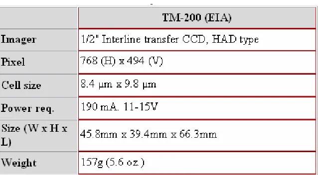
The developed face database (indoor at the laboratory) are acquired through a single monochrome camera and embedded frame grabber see figure 5. The system uses PULNiX TM-200 camera that offers a high resolution interline transfer 1/2" CCD imager in a very tiny package. Designed to meet a variety of application requirements, this camera has many standard and optional features. It is available in both EIA (TM-200) formats. The most commonly needed adjustments-manual gain, gamma, AGC, and field/frame selection-are easily accessible on the rear camera panel. Eight shutter speeds, ranging from 1/60 sec. to 1/10,000 sec., can be selected externally using the rotary dial on the rear panel. Table 1 shows some specifications of the device.

As for the frame grabber Matrox Meteor-II/Multi-Channel has been used, which has the following key features:

• PCI, CompactPCI® or PC/104-Plus™ form factor

• Captures from interlaced and progressive scan single or dual channel monochrome analog video sources

• Sampling rates up to 30 MHz

• Three 256 x 8-bit LUTs

• 32-bit/33 MHz PCI bus-master

• real-time transfer to system or VGA memory

• extensive on-board buffering for reliable capture

4 PRE-PROCESSING PHASE

As stated before, the preprocessing step is very critical yet essential task. Due to noise introduced from the electronic signals of the digital camera, face images may experience some resulted pixels that do not reflect the scene. Lighting uneven effect is also another intruder. In addition to these, an image analyzer might want to reduce the impact of the background on the objects (faces), by filling up small holes or make them to vanish, this will of course depend solely on the purpose of the algorithm. Here, the next sections will bring about some famous and strong preprocessing techniques that have been used.

4.1 Histogram Equalization

Lighting conditions have an enormous effect on the segmentation too. That is why when matching faces; the conventional techniques based on correlation between gray levels are proven to be impractical, because intensity values are prone to change by different factors. Since a face illumination from the left looks different than that from the right, therefore, the image windows must be corrected for illumination. Generally, illumination effects tend to behave as a linear ramp. Thus a solution was needed. A simple way yet powerful to ameliorate the problem is by applying

“Histogram Equalization”, which is described beneath:

It mainly enhances the contrast of images by transforming the values in an intensity image, or the values in the color-map of an indexed image, so that the histogram of the output image approximately matches a specified histogram or the one can see it as generating a flat histogram. This transformation transforms the intensity image I so that the histogram of the output intensity image let say J with length A bins approximately matches

A

A

A

where n denotes number of bins.

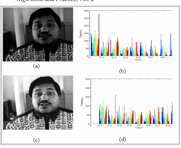
Figure 6 Histogram Equalization (a) Original BioID face image (b) its respective histogram (c) resulted image and (d) its respective histogram. Note the images were in double precision and there intensities values range from 0 to 1

4.2 Applying Morphological Operations

Given an image I and structuring element

ψ

ψ

ψ

Then the Erosion of I by

ψ

I

Θ

ψ

Δ

{

x

:

ψ

⊂

I

}

Similarly the dilation of I by

ψ

I

⊕

ψ

Δ

{

x

:

ψ

∩

I

≠

φ

}

Therefore the opening is the combination stated as follows:

=

ψ

D

I

(

I

Θ

ψ

)

⊕

ψ

A square structuring element with size of 2 has been used, Figure 7 gives a practical example.

Figure 7 Opening process (a) Histogram equalized image (b) Result of opening with square size 2 (c) The hit places by the opening and (d) The effect on the face feature (bright in the right eye of (a) is filled).

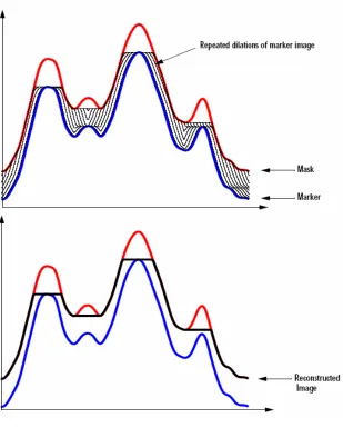
The marker can be constructed easily and straightforward by subtracting a value from the original image.

5 FACE SEGMENTATION

In what follows, a novel method for locating and extracting face/head boundary is introduced. As it is mentioned earlier the preprocessing stage plays a major role in segmentation process. During this stage, the image illumination must be distributed evenly; edges must be smoothed and linked to ease the extraction of contours.

As it is shown in the system overview section, a dual processing scheme has been followed. That is the Voronoi is applied on feature points of the origin image and its complement as well. Although it doubles the time consumed but on the other hand it’s found to be very efficient to ease the task of segmentation. It is especially useful when having the problem of intensity similarities between the face and its background. The author emphasizes here on the fact that each path of this dual scheme will not yield the perfect segmentation always; therefore a rule is based to chose between the outputs of the two.

5.1 Definition of Vd And Dt

from these two input points. A Voronoi vertex is an intersection of Voronoi edges and is associated with three (or more) input points such that each Voronoi vertex is equidistant from these input points as shown in.

More formally, let a set S = {p1; : : : ; pn} of n distinct points in the plane. The Voronoi cell V (pi) of a point pi

∈

}

),

,

(

)

,

(

:

{

:

)

(

p

q

d

p

q

d

p

q

i

j

V

=

∈

ℜ

≤

≠

Here, d (p;q) denotes the ordinary Euclidean distance between p

and q

2

2

₍

₎

)

(

x

−

x

+

y

−

y

The Voronoi diagram V (S) of S is the family of subsets of

2

ℜ

∈

ℜ

Figure 9 The Voronoi diagram of some points 1; : : : ; 7

Here the Voronoi is constructed on a finite set of distinct sites in the Euclidean space; which means that these points are not supposed to be collinear. In addition to this the minimum number of points is set to four points (sites). Voronoi diagram has several properties which are listed beneath:

• The nearest generator for all the points in the Euclidean subspace defined by V (gi) is gi (this is the definition of Voronoi diagrams).

• A Voronoi diagram is a unique tessellation.

• Every Voronoi region V (gi) is a non-empty convex polygon.

• A Voronoi polygon is infinite if and only if its generator is on the convex hull of the generators set.

• All Voronoi edges are straight lines of infinite extend if and only if the generators are collinear.

• The closest generator to gi generates one of the edges of the Voronoi region V (gi) (and hence they share the edge).

• The Voronoi diagram of a set of n point sites in the plane has at most 2n-5 vertices and 3n-6 edges.

• A point q is a vertex of V(S) iff its largest empty circle C(q) contains three or more sites on its boundary and there is no site located inside the circle(M. Berg, 2000; A. Okabe et al., 2000)

• The union of all borders of the voronoi cells V (P1),

V (P2), …., V(Pn) constitutes the Voronoi diagram

The properties of Voronoi polygons draw the attention of many researchers; as a result various algorithms have been developed to calculate the Voronoi, the reader is directed to any geometry book. Among these methods are Divide and Conquer Algorithm, Fortune’s Algorithm (Seul M. et al., 2000) or what Trigui A. (2002) described as Fortune Plane Sweep algorithm and region growing (Ahuja N., 1982).

Table 2 Shows the difference between Voronoi and Fixed Radius approaches

Voronoi Diagram Approach Fixed Radius Approach

• The Voronoi

tessellation assigns each region of the plan to the neighbor of one and only one point.

• The set of circles of radius R centered at a given set of points will, in general, have regions of overlap. There will be also regions surrounded by various

neighborhoods but not included in any figure 10

Table 3 shows the difference between Voronoi and K.NN

approaches

Voronoi Diagram Approach K-Nearest Neighbor Approach

Some point’s neighbors may be far away from it than some other points which are not Voronoi neighbors figure 11.

Figure 10 The fixed radius weaknesses

The dual tessellation of the Voronoi Diagram (VD) is known as Delaunay Triangulations (DT) Figure 12 in the following sense: vertices in the Voronoi diagram correspond to faces in the Delaunay triangulation, while Voronoi cells correspond with vertices of DT. Once the Voronoi diagram for a set of points is constructed it is a simple matter to produce Delaunay triangulation by connecting any two sites whose Voronoi polygons share an edge. Or in another way, let P be a circle free set. Three points Pi, Pj, Pk of P define a Delaunay triangle iff there is not further point of P in the interior of the circle which is circumscribed to the triangle Pi, Pj, Pk and its center lies on a Voronoi vertex, Figure 13 depicts this notion.

Figure 13 pqr define a Delaunay triangle when the center (s) of the circle circumscribed to pqr is a Voronoi vertex

Delaunay Triangulation as far as geometry is concern has some properties which are listed below:

• The external triangle edges of the Delaunay tessellation is the convex hull containing the given set of sites.

• It is the dual tessellation of the Voronoi diagram.

• There is no site located inside the circle passing through the vertices of any Delaunay triangle.

5.2 Application of Vd/Dt

There is a wide variety of geometric problems that can be naturally solved using spatial tessellations which explains why they are so widely used in many different applications. More specifically,

θ

p

q

s

given a set of points, some of the problems that the Voronoi diagrams can solve, efficiently, are:

1. The closest pair problem.

2. The all k nearest neighbors’ problem. 3. The all nearest neighbors’ problem. 4. The fixed radius near neighbors.

5. The nearest-search problem (the "Knuth's Post Office problem").

6. The largest empty circle problem (the "Toxic Waste Bag problem").

The proposed approach is based ultimately on Voronoi Diagram (VD) technique, which is a versatile geometric structure (Costa L. and Cesar R., 2001; Ahuja N., 1981, Xiao Y. and Yan H., 2002). In spite of its usefulness in various fields ranging from Remote Sensing to Robot Navigation, this method was largely forgotten in applications in image segmentation until Suhail M. et al., (2002) rekindled interest in it. Their approach was based on extracting feature points, which they used to define Voronoi cells’ centers for image segmentation. The researcher proposed method although it is inline with theirs in using VD; however the proposed way and target are completely different.

Figure 14 CPU times for computing Delaunay graphs on SUN SPARCstation 10/20 (Reinelt G., 1994)

So, VD is constructed from features points (generators) which result from gray intensity values summations (frequency).

∑ = ∑= =m

i n

j f x y k x

Val

1 1 ( , ) )

( (15)

Where

k is the range of the intensity values, k= {0, 1, 2….255}, and f(x, y) denotes pixel location in the host image.

The method has the spirit of dynamic Thresholding used for segmentation while it differs in terms of divide and merge decision. Human faces have a special color distribution that differs significantly from that one of the background. The VD is used to

construct the Delaunay Triangulations (DT). The outer boundary of DT is simply the convex hull of the set of the featured points. The convex hull CH(S) of a set of points is the smallest convex set containing these points. It is a convenient means for representing point sets. If the point set is dense then the convex hull may very well reflect its shape. Large and diverse instances ones usually exhibit several clusters. Building the convex hull of these clusters can result in a concise representation of the whole point set still exhibiting many of its geometric properties. Many algorithms were introduced to build the CH(S) e.g.: Graham’s Scan, Divide and Conquer, Throw-Away Principles and Convex Hulls from Maximal Vectors.

Hence by getting the CH(S) the global two maxima are obtained. In order to get the minima that fall between these two peaks, a new set of points are generated using the following steps:

• Generate the host image histogram

• Set all the points below the first peak to zeros, and set all the points beyond the second peak to zeros.

• Set all points that are equal to zeros to be equal to the argmax (peak1, peak2).

• Derive the new points by:

||

)))

(

max(

)

(

(

||

)

(

x

val

x

val

x

Val

=

−

(a)

(b)

It should be born in mind that the outer layer of DT contains vertices which are but some selected Voronoi (VD) generators, in another word the vertices forming the CH are what the study is interested in. In this case these vertices give a direct access to their respective gray values Figure 16.

Figure 16 Delaunay Triangulation being imposed on the histogram of figure 15a

Input: Host gray scale image

Ψ

Input: Vector generated by the previous described procedure

Ω

Set all pixels in

Ψ

Ω

(

1

,

1

)

Set all pixels in

Ψ

Ω

(

length

(

Ω

(:)),

1

)

for i = 1 to

length

(

Ω

(:))

−

1

set all (

Ψ

Ω

(

i

)

Ψ

Ω

(

i

+

1

)

Ω

(

i

+

1

)

Ω

(

i

+

1

)

else

set all (

Ψ

Ω

(

i

)

Ψ

Ω

(

i

+

1

)

Ω

(

i

+

1

)

Ω

(

i

+

1

)

end if end for

Output segmented gray scale image

Ψ

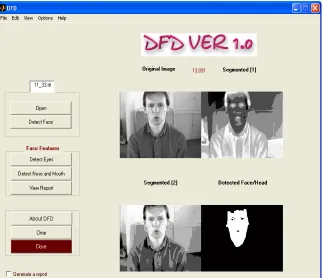
Figure 17 Segmentation using the proposed method. (a) Original image (b) Segmentation based on the image complement (c) A direct segmentation and (d) (c)-With colormap

Table 4 Shows the benefit of segmentation in gray values’ reduction (re-sampling)

To conclude this section, the author stresses that although the scope of this research is bounded by face database with gray scale images, however the designed system can handle the segmentation of other types of images as it is clear from the next example figure 18.

A second fact is that the Voronoi based image segmentation can be extended to RGB images without converting it into grayscale, that is done by working on the RGB map only and treating each color matrix as a separated input to the segmentation process.

Figure 18 Application of the algorithm on WWW images. The method can be extended to non face images. Up to this point the algorithm is general

5.3 Extraction of Probable Face Region

any block less than an arbitrary value by disregarding all blocks less than (60*60); many authors in the literature have chosen this size of window as the minimum size of the face. A labeled image is defined as:

k G y x f y x

h^( , )=∀ ( , )∈ (17)

where

Gk is a labeled region, and k is the number of segments.

Hence, each binary segment

δ

⎩

⎨

⎧

∈

=

otherwise

G

y

x

f

if

n

₀

_,

)

,

(

,

1

δ

It has been found that faces show elliptical shapes with minor variations in eccentricity from one person to another. The ramp transition characterizing the face intensity will give a hand, because in general it forms a contour of on pixels surrounding off

pixels, which means when filling it the exact shape of the face is obtained. Thus, the voting phase can be made based on detection of ellipses.

To cope with this situation, the distance transformation (DisT) is introduced to separate the face region from its background. The function operates on the Euclidean distance between two given points (x1, y1) and (x2, y2), where:

2 ) 2 1 ( 2 ) 2 1

(x x y y

DisT= − + − (19)

Then a new image is chosen obtained by the following:

new_image=(DisT>=Th) (20)

where

Th denotes a threshold value. The resulted image is dilated with a structuring element of size 3 in order to recover back the shape distorted by the DisT function.

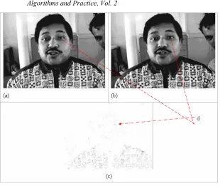
Figure 19 Applying Distance Transformation to cut the bridge merging the face with the background. (a) Original image (b) Segmented (complement) (c) filled segment (d) Its DisT and (e) Background eliminated

As a vivid example on the DisT in binary images and its concept, let’s have a small matrix (5*5) and name it bw:

bw = 0 0 0 0 0 0 1 0 0 0 0 0 0 0 0 0 0 0 1 0 0 0 0 0 0

The associated values of the DisT from the off pixels to the nearest

DisT = 1.4142 1.0000 1.4142 2.2361 3.1623 1.0000 0 1.0000 2.0000 2.2361 1.4142 1.0000 1.4142 1.0000 1.4142 2.2361 2.0000 1.0000 0 1.0000 3.1623 2.2361 1.4142 1.0000 1.4142

Since horizontal and vertical pixels of 8 neighbor point have the distance of 1 unit, the diagonal direction however has the distance

of

1

+

1

=

2

=

1

.

4142

After stepping out from this probable problem, three main criterions for a possible rule can be used for estimating and evaluating the Region Of Interest(ROI), which are:

• Rule 1: Ellipse Fitting

This is a well known strategy for face estimation and segmentation. The connected components given by the above stage will be fit into an ellipse model. An ellipse is ultimately characterized by its center (X0, Y0), Orientation (θ), minor axis (a) and major axis (b). The center is but the center of mass, while θ is determined using the least moment of inertia:

))

(

2

arctan(

2

/

1

M

M

−

M

=

θ

where

Mi ,j denotes the central moments of ĥ (x ,y).

∑

∈ − − − =

C y

x, ) x X y Y

( 2 ] sin ) 0 ( cos ) 0 [( min

I θ θ (22)

∑ ∈ − − − = C y x Y y X x ) , ( 2 ] cos ) 0 ( sin ) 0 [( max

I θ θ (23)

8 / 1 ] min / 3 ) max [( 4 / 1 ) / 4

( I I

a= π (24)

Assessing how well the ĥ (x, y) is approximated by its constructed ellipse the new distances measure is defined between ĥ (x, y) and the best fit ellipse as fellows:

фi=p_inside/M_0,0 (26)

0 , 0

/M

outside

p (27)

Where

Pinside denotes the sum of background pixels within the ellipse, Poutside is the sum of ĥ (x, y) pixels lying outside the ellipse (Haddadnia J. et al., 2002), and M0,0 is the total area of ĥ(x, y).

• Rule 2: Cross Correlation

This is an acknowledged strong method in detecting objects and reporting the level of much. It is well know that in binary images Cross Correlation has less computational complexity comparing to gray scale. Therefore the study came up with the model depicted in Figure 20.

Figure 20 Template model to vote for face blocks

A binarized face region will expose face features as holes because of their low intensity. This helps in judging a probable face region in terms of its Euler number. Therefore, it is safe to say that a face would consist of at least two holes. To determine that, the following equation is used:

H

C

E

=

−

where

E is the Euler number, C is the number of connected components and H is equal to the number of holes. Because only one segment is present at a given time, the value C is equal to one. Thus,

E

H

=1

−

In this research Rule2 and Rule3 are selected to judge any segment whether it contains a face.

REFERENCE

COSTA L.AND CESAR R., 2001. Shape Analysis and Classification, CRC Press, USA.

DOWDALL J.,PAVLIDIS I.AND BEBIS G., 2003.Face detection in the near-IR spectrum, Elsevier Sci. Image Vision Comput.

vol.21, pp. 565–578.

H. Dang and D. Claussi, (2004). Unsupervised image segmentation using a simple MRF model with a new implementation scheme. Pattern Recognition 37 (2004) 2323 2335

HADDADNIA J.,AHMADI M.AND FAEZ K., An efficient method for recognition of human faces using higher orders pseudo Zernike moment invariant, IEEE Proc. Fifth Int. Conf. Autom. Face Gesture Recognition, pp. 315–320.

HSU R.AND ABDEL-MOTTALEB M., Face detection in color images,

IEEE Trans. Pattern Anal. Mach. Intell. Vol.24, no.5, pp. 696– 706.

KWOLEK B., 2003. Face tracking system based on color, stereovision and elliptical shape features, IEEE Proc. IEEE Conf. Adv. Video Signal Based Surveillance, pp. 21–26.

N. Ahuja.(1982). Dot Pattern Processing Using voronoi Neighborhoods. IEEE Trans on Pattern Recognition and Machine Intelligence. PAMI-4.3. 336-343

RIZON M. AND KAWAGUCHI T., Automatic eye detection using intensity and edge information, Proc. IEEE TENCON vol.2, pp. 415–420.

SEUL M., O’GORMAN L. AND SAMMON M., 2000. Practical

Algorithms for Image Processing, Cambridge University Press, USA.

XIAO Y. AND YAN H., 2002. ‘Facial Feature Location with

Delaunay Triangulatiod Voronoi Diagram Calculation’. Australian Computer Society, Inc. The Pan-Sydney Area Workshop on Visual Information Processing (VIP200 1).