An unconditional maximum likelihood test for a unit rood

Dy

Gracicla

Gon7.a.lC'~-Farias and David A. Dickey

Insti tute of Statistics

Mimm

Serics

#~ ~:l"'.~

Jannary, 1992

~

~"'S

NAME

LIKELIHOOD TEST FOR A UNITI

ROOT

DATE

I

I

l

The

Library of

th

N

e

Department

of

Star r

....

..

AN UNCONDITIONAL MAXIMUM LIKELIHOOD TEST FOR A UNIT ROOT

Graciela Gonzalez-Farias and David A. Dickey

North Carolina State University Raleigh, North Carolina

Key Words: Time Series, Nonstationary

Abstract

We investigate a test for unit roots in autoregressive time series based on maximization of the

unconditional likelihood. This is the likelihood function appropriate for stationary time series. While

this function is the true likelihood only under the stationary alternative, it can nevertheless be

maximized for any data including data from a unit root process. It thus gives a way to test for unit

roots, provided percentiles can be calculated. For models with estimated means, the power of the new

test is better than that of some currently popular tests.

1. INTRODUCTION

Time series modeling often involves the selection and fitting of an ARIMA (autoregressive

integrated moving average) model. The order of integration is defined as the degree of differencing

required to make the series stationary where stationarity implies constant mean and variance over time

and a covariance which depends only on the time separating two observations. The fitting of a series

traditionally involves differencing the data if necessary, until they appear stationary then fitting

autoregressive and moving average parameters to the, possibly differenced, data. We investigate

statistical ways to check whether differencing is necessary.

Appropriate differencing renders a series stationary and thus makes the resulting estimation theory

easier to work out. The results tend to be classical in nature, for example normal limit distributions of

estimators. Classic methods of estimation, such as least squares and maximum likelihood are not

necessarily poor estimation methods for the parameters of nonstationary series, however the

distributions are not standard even in the limit. Ifpercentiles of the distributions can be obtained,

For ARIMA models, stationarity can be characterized by a condition on the roots of a polynomial

involving the autoregressive coefficients, called the characteristic polynomial. Ifall the roots are larger

than 1 in magnitude, the series is stationary. Therefore we can base a test for stationarity on the

coefficients or roots of the characteristic polynomial. These in turn must be estimated in some way.

Such tests are often called unit root tests (unit roots being the null hypothesis) but could arguably also

be called tests for stationarity when that is taken as the alternative. The most important motivation

for developing a test for stationarity is that certain economic hypotheses are mathematically equivalent

to stating that there are unit roots in the corresponding data series.

Tests based on least squares estimation are reasonably well known. Least squares maximizes the

likelihood conditional on the initial observation(s). This is in contrast to the unconditional likelihood

function for a stationary model that is used by computer programs written to do maximum likelihood

analysis. This unconditional likelihood function can be maximized regardless of the true nature of the

data and thus might be thought of as an objective function rather than a likelihood. Under the

alternative hypothesis of stationarity, such an estimator should do well. However, it is not clear how

well it would perform under the null hypothesis of a unit root nor is it clear what the distribution of

the unconditional maximum likelihood estimator would be in this case.

We show that the distribution in question is nonstandard and differs, even in the limit, from that

of the least squares estimator. Further, this new estimator has superior power in some instances of

practical interest.

2. TEST CRITERIA, MEAN KNOWN (/1

=

0)

While the case of a known mean is of little practical value, the algebra is simple and the ideas of

the proof carryover to the more practical cases. In what follows, we outline the main steps of the

..

details.

Hasza (1980) and Anderson (1971, pg. 354) study the AR(1) case with known mean using the

stationary likelihood function. They show that the maximum likelihood estimator of p in the model

Yt

=

pYt-1

+

et, et ,....,

N(O,17

2) can be written as the solution

p

to the cubic equation g(p)

=

0where

_ (n - 1 n-l 2) 3 (n _ 2 n-2 ) 2 (n-l 2 1 n 2) ( n )

g(p) - - n - E _{Yt p - -n- E YtYt-}1 p - EYt

+

ii EYt p+ EYtYt-1

t=2 t=2 t=2 t=l t=2

Using the formula for the roots of a cubic equation, a closed form solution can be given (see Hasza,

1980).

Although this gives a neat solution in the first order case, we want to look at higher order

1n-l

processes. Let X

=

n(p - 1) and divide g(p) by n -; E Y~. The result is

n t=2

where

p

=(

~y~)-l(

t

_YtYt-1) which is almost exactly the ordinary least squares estimator and

t=2 t=2

15

=

[~(Yi

+

Y~)

+

~ y~Jl

[t

_YtYt-1] which is the symmetric estimator as defined in Dickey,

2\

t=2 t=2

Hasza, and Fuller (1984). Both n(p -1) and n(p-1) are Op (1). Since the leading coefficient in qn(X)

is l/n, we see that the probability limit of the polynomial qn(X) over any closed X interval is the same

as the probability limit of the quadratic

Q(X)

=

2X2- 2[n(p - 1)] X

+

2[n(p - 1)]. (2.1 )

13ecause of the Op (1) order of the random coefficients and the fact that n(p -1) is strictly negative, we

can find a closed X interval such that with arbitrarily high probability for a given {y

>

0, the roots of

qn(X) are real, the largest two are within the closed X interval, and these two are within {y of the roots

as the maximum likelihood estimator.

Using the notation of Dickey and Fuller (1979) we define

• 2 n 2 -1 n

(r,()

=

hm (n _{EWt_1,} n _{EWt_1Zt)}

n-+oo t=2 t=2

where W t is the random walk defined by Wt

=

_{W t_1}

+

Zt and Zt ... N(O,

1).

Alternatively, Chan and Wei define

(r, ()

as

(J

5

W2(t)dt, !(W2

(1) -1))

where Wet) is Brownian Motion. The limit of

expression (2.1) in terms of

(r, ()

becomes

(2.2)

Techniques described in Dickey (1976) can be used to simulate the random vector

(r, ()

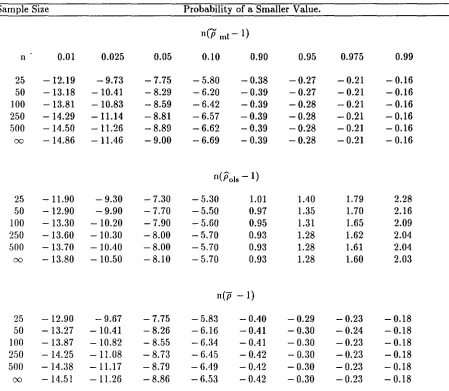
from which

the roots of(2.2) can be found, and percentiles tabulated. Table 2.1 contains percentiles of the

unconditional maximum likelihood estimator's distribution for finite samples and the limit. These are

labelled n(ffml - 1). Also listed for comparison are the least squares estimate n(pol_{s -} 1) as in Fuller

(1976) and the symmetric estimator n(p -1) as in Dickey, Hasza, and Fuller (1984). Gonzalez-Farias

Table 2.1. Empirical cumulative distribution of the estimators ofp, p=1.

Sample Size Probability of a Smaller Value.

n(Pml- 1)

n 0.01 0.025 0.05 0.10 0.90 0.95 0.975 0.99

25 -12.19 -9.73 -7.75 -5.80 -0.38 -0.27 -0.21 -0.16

50 -13.18 -10041 -8.29 -6.20 -0.39 -0.27 -0.21 -0.16

100 -13.81 -10.83 -8.59 - 6042 -0.39 -0.28 -0.21 - 0.16

250 -14.29 -11.14 -8.81 -6.57 -0.39 -0.28 -0.21 -0.16

500 - 14.50 - 11.26 -8.89 -6.62 -0.39 -0.28 -0.21 -0.16

00 -14.86 - 11.46 -9.00 -6.69 -0.39 -0.28 -0.21 -0.16

n(poi_{s -} 1)

25 - 11.90 -9.30 -7.30 -5.30 1.01

lAO

1.79 2.28

50 -12.90 -9.90 -7.70 -5.50 0.97 1.35 1.70 2.16

100 - 13.30 - 10.20 -7.90 -5.60 0.95 1.31 1.65 2.09

250 -13.60 -10.30 -8.00 -5.70 0.93 1.28 1.62 2.04

500 -13.70 - 10040 -8.00 -5.70 0.93 1.28 1.61 2.04

00 -13.80 -10.50 -8.10 - 5.70 0.93 1.28 1.60 2.03

n(p -1)

25 -12.90 - 9.67 -7.75 -5.83 - 0040 -0.29 - 0.23 - 0.18

50 -13.27 - 10.41 -8.26 -6.16 - 0.41 -0.30 -0.24 - 0.18

100 -13.87 -10.82 -8.55 -6.34 - 0.41 -0.30 -0.23 -0.18

2.50 - 14.25 - 11.08 -8.73 - 6.45 - 0.42 - 0.30 -0.23 -0.18

500 -14.38 -11.17 -8.79 - 6.49 - 0.42 -0.30 -0.23 -0.18

The limit distribution does not change if additional lags are included in the model. This will also

be true in the case where the mean is estimated. To illustrate this result, consider a second order,

AR(2), model. The AR(2) model with mean 0can be written as

Yt = (ml + m 2) Yt-l - mlm2 Yt-2 + et

and the logarithm of the stationary likelihood for e_t normal is

where the sum of squares SSQ is

SSQ = f:(Y_t-(m_{l +m2)Yt-1}+m_lm2y_{t_2)2} t=3

SlIppose the true value of (ml , m2) is (1, 0') with 10'1

<

1. Now let X = n(ml -1) and S = Jll(m2 - 0')

and consider the function En(L) for (X, S) in an arbitrary closed rectangular region R. Let;:;2 denote

the maximum likelihood estimator ofu2for any given (X, S) and note that for (X, S) in R we have

since, in R, m_l = 1 + O(I/n) and m2 = 0' + 00/ Jll). Substituting;:;2 into En(L) we have the

concentrated likelihood

€n(L) = - (n/2)€n(;:;2) + (1/2)€n( - X/n) - (n/2)€n(2II)

+ (1/2)€n[0 + m_t)(1 -

m~)(1

- m_{tm 2)2] - (n/2)}

Only the first two terms affect the limit distribution. In fact the X=n(m_{l - 1) and S=Jll(m2 - 0')}

which maximize €n(L) are asymptotically the same as the (X, S) which maximize

Fn(X, S) = [ - (n/2)€n((SSQ)/n)] + (1/2)€n( - X) + C (2.3)

where C is constant with respect to X and S. See Gonzalez-Farias (1992 appendix B). For (X, S) in R

we have

SSQ = f:[e_{t -} X (Y_{t- l -} O'Y_{t _2})/n - S(Y_{t _1 -} Y_{t - 2 )/}Jll + XS(Y_{t _2}/n3/2

)f

3

Notice that XS in SSQ is multiplied by n-2 Y_t-_{2, a term whose sum of squares converges to}O.

Furthermore l{(Y_{t -t -}

aY

_{t_}2

)/n

(Yt -t -

Y

t-2

)1

yn]

converges to 0. In the limit, then, the log likelihood

is the sum of two functions, one involving only S and one involving only X. Specifically, SSQlu2

-n

L:

e~

I

u2 is a polynomial in (X, S) and converges uniformly in Rto

t=3

[ - 2X(

+

x

2

r]

+

[S2/(1 - ( 2) -

2 SV] (2.4)

whereV '" N(O, (1 - a2rt). The derivatives ofSSQlu2also converge to the derivatives of(2.4). This

result follows from the well known rates of convergence of sums of squares and cross products for

st,ationary and unit root processes. Taking the derivative, with respect to X, of Fn(X, S), we see that

the limit maximum likelihood estimator satisfies

or

2X2- 2((/r)X

+

2(

2f)

=

°

which is the same as (2.2). Note also that taking the derivative of Fn(X, S) with respect to S gives the

same limit normal distribution for

yn(m

_{2 -} a) that would be obtained from applying least squares or

maximum likelihood to the model

Since the region R can be any closed rectangular region with (X, S)=(O, 0) an interior point, the orders

of sums of squares and cross products in

(2.3)

imply that, given any 8

>

0, the (X, S) which maximizes

F_n is eventually within this region with probability at least (1 - 8). Over R, the function

en(i) - Fn(X, S) converges uniformly to 0, so the normalized maximum likelihood estimates of mt and

m2 converge to the maximizing (X, S).

We have outlined the case of the known mean since the algebra is relatively easy to follow and

involves only a few terms. In the next section, we look at the more practical case in which the mean p

is estimated. The main ideas are similar to the case just presented, but the algebra is more tedious

3. TEST CRITERIA, MEAN ESTIMATED

Consider the model for Yl' ..., Yn

Y_t = J.l(1- p)+pY_t-1+e_{t ,} t=2, 3, ... ;Ipl

<

1

where e_t is a sequence of iid N(O, 0-2) random variables. We will study the model (3.1) under two scenarios, namely, Y₁being fixed and

3.1. Case 1: Y₁fixed.

When Y1is considered fixed, the estimator ofp is obtained by maximizing the log likelihood

function conditioned on Y₁, namely

(3.1)

1

20-2

(3.2)

This is commonly called the conditional maximum likelihood estimator. IfJ.l is estimated, the

conditional maximum likelihood estimator is also asymptotically equivalent to the ordinary least

sqlJares estimator

P"

ols ofp, obtained by regressing Y_t on 1 and Y_t-1. Asymptotic properties ofPols

r' IJ,

when p

=

1 have been very well established in the literature, see for example, Dickey and Fuller (1979).

The estimator's distribution does not depend on the value of Jl in (3.1).

Dickey and Fuller (1979) show that the pivotal statistic

2 1 n -2 - _ 1 n

where S

=- -

2:

e_t and Y(-1) - n _ 1

2:

Y_t-1and T" can be expressed as a function of standard

normal variates. Again this statistic does not depend on the true value ofJ-l in (3.1). In fact, adding a

constant c to every observation has no effect on either

P

/-l,oIsor T/-l' Table 8.5.2 of Fuller (1976) gives

the percentiles of the TJ-l distribution.

3.2. Case 2: Y1 '" N(J-l' (72 / (1 _

p2)) .

Consider n observations Yl' " ' , Yn from the model (2.1). Then, the log likelihood function is

given by

\vhere i *(J-l' p, (72)

= -

~

log 211 -

~

log (72

+

!

log (1-p)

For any given p and (72, both i and L* are maximized at

(3.3)

n-l

Y1

+

Yn - (p - 1)

L:

Yt

jl(p)

=

2-(n-2)(p-l) (3.4)

- 1

where Y1

=

n _ 2

Notice that jl(p) is a weighted average of the data so that any statistic defined as a function of

Y_I- iJ(p) will be unchanged by the addition of a constant c to every observation. This shows that

such a statistic is independent of the value ofJ-lin (3.1).

Let iJ,~, P~ and (7~2be the values ofJ-l, p and (72 that maximize L*. Itis shown in

Gonzalez-Farias (1992) that the asymptotic distribution of(jl* ,_m p* , 0'*2)_{m m} is the same as (iiml'

P

_ffi,rnI' (72_ID,IDI) the maximum likelihood estimator of(J-l, p, (72), so it is sufficient to use L*as the objective to maximize.

THEOREM. Suppose Y_t

=

Y_{t -1}

+

e_t where e_t is a sequence of iid (0, (7~) random variables with

that maximize L*(Il, P, (T2). Then

and

(_n(jJ~

n-~

jl:U)

-

₁₎

1

(H

A

:)

0-*2

=

1

~

e2

+

0 (1)

m n t~2 t p n

(3.5)

where H* = H + T - 2H and A* is the unique negative solution to 2-A*

(3.6)

The a/s are funetionals of a standard Brownian motion W(t). Following Dickey and Fuller (1979),

and Chan and Wei (1988), (f, H, T)

=(J~W2(t)db, J~W(t)dt,

W(I)).

Let fIl = f - H2, (=!(T2-1), and (,. = ( - TH. Then

a4

=

2fp' a3

= -

2((1l

+

H 2

) - 8f,.,

a₂

=

8f1l+8((fJ

+

H2)-1 ,

a₁

= -

8((fJ+ H2) + 2(T - 2H)2 + 4, aD = - 4.

Proof: We present here a sketch of a proof. A detailed proof appears in Gonzalez-Farias (1992).

Taking partial derivatives ofL* with respect toIl, and (T2 and setting them equal to zero we get

jl~

=

!i(jJ:U)

and

iJ:u

is a solution to

a* f3-*4+ a * iJ*3+ a * f3-*2+ a *

jj*

+a* = 0

4m m 3m m 2m m 1m m Om

(3.7)

(3.8)

a~,n

= -

4

+

oi)n)'

r

-

1

n,I' - n2

and

The coefficients a:"_I,n in (3.9) converge jointly in distribution to the coefficients aj in (3.6).

By Theorem 13.8 of Breiman (1968), we can change to a new probability space on which

{ai,n'

i

=

0, " ' , 4}

.E{aj,

i

=

0, " ' , 4}.

The limit polynomial given in (3.6) can be factored giving

and hence, we can show that it has a unique root X=A

*

in ( - 00, 0).

Also, since a:"_l,n= Op(I), i=O, ... , 4 and a₄*_tn and a₄ are positive random variables, it is possible to

show that with a very high probability the polynomial in (3.9) has a solution,

p:n

in the interval

( - n, 0).

Then, using the Implicit Function Theorem we get that with high probability, there exists a

unicJlle

P;n

that satisfies (3.9) and is a continuous function of ai,n,i=0, .. ·,4 and hence

P:U

.1A*.

Note that, the partial derivative of1.(/J,p,0"2) is

~~

=

2(I~P)

+

81.*(JJ

a;,

0"2))

After some algebra we get that the maximum likelihood estimator ofp, or equivalently

~~l=

n(p:U,

ml - 1) is a solution to a fifth degree polynomial,

5 _.

2:

a· j31

=

0

. l,n m 1=0

Note that the polynomial in (3.10) behaves similarly to the fourth degree polynomial we obtained

for 1.,*and hence the asymptotic distribution for the maximum likelihood estimator is the same as that

of(iI.*_rm' p'*_m' iT*2)._m

4. Remarks

1. The maximum likelihood estimators may also be obtained iteratively. For a given

Pj

- 1 and iT?-1'

h

may be obtained from (3.4). For a given

P'i'

we then obtain

Pj

and iT? by maximizing L(jti' p, (72).

It, can be shown that

p.

is a solution to a cubic equation where the observations are centered at ji,. and

I I

a closed form expression is given in Hasza (1980).

2. When we assume that 1"=0in the model (3.1) then the MLE ofp that maximizes 1.,(0, p, (72) is

obt.ained by solving (2.2), namely

• GJ _

If (

(2

2

1/2}

n(Pml - 1) -+ A -

21.

r - {

r2

+

r}

.

An empirical study that. compares the powers ofPolsand Pmlindicates that there are essentially no

differences in the power among these test criteria in the1"=0 case.

~. A Wald type pivotal t-statistic can be constructed for testing p=l,

(p -1)

JV(p)

where V(p) is determined from the negative matrix of the second derivatives of the corresponding objective function.

tl. For the higher order processes, we consider the model

(3.11)

where Zt is a stationary AR(p -1) model, 1

>

P~ max Imjl and mj' i

=

2, . ", p are the roots of the

characteristic equation of the Zt process. Using methods similar to those in section 2, Gonzalez-Farias

model (3.11), is the same as that of

n(P

_m,

ml)

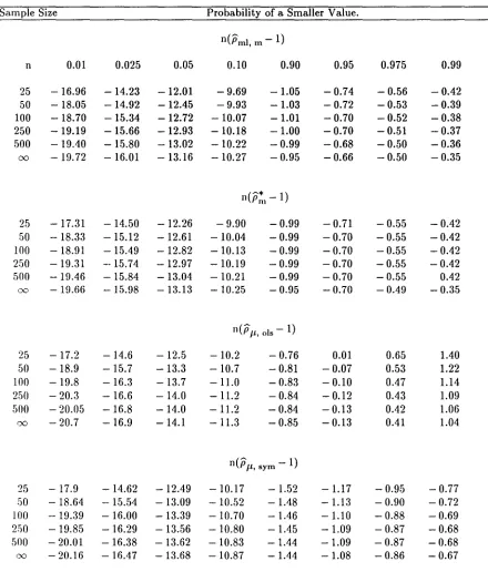
derived for the AR(1) case.

Tables of percentiles for the different estimators mentioned above are given in Table 4.1 4.2.

The top panel of each table is the maximizer ofL(j.l, p, 0-2)and the second the maximizer of

L*(j.l, p, 0-2) as in (3.3). The last two panels are the least squares and symmetric estimators as in

Table 4.1 Empirical distribution of the normalized bias estimators.

Sample Size Probability of a Smaller Value.

n(Pml, m - 1)

n 0.01 0.025 0.05 0.10 0.90 0.95 0.975 0.99

25 -16.96 -14.23 -12.01 -9.69 -1.05 -0.74 - 0.56 - 0.42

50 -18.05 -14.92 -12.45 -9.93 -1.03 - 0.72 -0.53 -0.39

100 -18.70 -15.34 - 12.72 -10.07 -1.01 -0.70 -0.52 -0.38

250 -19.19 -15.66 -12.93 - 10.18 -1.00 -0.70 -0.51 -0.37

500 - 19.40 -15.80 -13.02 -10.22 -0.99 -0.68 -0.50 - 0.36

00 - 19.72 - 16.01 - 13.16 -10.27 -0.95 -0.66 -0.50 - 0.35

n(p~l-l)

25 - 17.31 -14.50 -12.26 - 9.90 -0.99 -0.71 - 0.55 - 0.42

50 - 18.33 - 15.12 -12.61 -10.04 -0.99 -0.70 - 0.55 -0.42

100 - 18.91 -15.49 - 12.82 -10.13 -0.99 -0.70 -0.55 -0.42

2.50 - 19.31 --15.74 -12.97 -10.19 - 0.99 -0.70 -0.55 - 0.42

500 - 19.46 - 15.84 -13.04 -10.21 -0.99 -0.70 -0.55 0.42

00 - 19.66 -15.98 - 13.13 -10.25 -0.95 -0.70 - 0,49 -0.35

n(pj.L,ols-l)

25 -17.2 -14.6 -12.5 -10.2 - 0.76 0.01 0.65 1.40

50 -18.9 -15.7 -13.3 -10.7 - 0.81 -0.07 0.53 1.22

100 -19.8 -16.3 -13.7 -11.0 -0.83 - 0.10 0.47 1.14

250 - 20.3 -16.6 -14.0 -11.2 - 0.84 - 0.12 0.43 1.09

500 - 20.05 -16.8 -14.0 -11.2 -0.84 - 0.13 0.42 1.06

00 - 20.7 -16.9 -14.1 -11.3 -0.85 -0.13 0,41 1.04

n(pj.L,sym -1)

25 -17.9 - 14.62 - 12.49 -10.17 -1.52 -1.17 - 0.95 - 0.77

50 - 18.64 - 15.54 -13.09 -10.52 -1.48 -1.13 - 0.90 - 0.72

100 - 19.39 - 16.00 -13.39 - 10.70 -1.46 -1.10 - 0.88 -0.69

2.50 - 19.85 -16.29 -13.56 -10.80 -1.45 -1.09 - 0.87 -0.68

500 - 20.01 - 16.38 -13.62 -10.83 -1.44 -1.09 -0.87 -0.68

Table 4.2 Empirical distribution of pivotal statistics

Sample Size Probability of a Smaller Value.

t

_ml,m

n 0.01 0.025 0.05 0.10 0.90 0.95 0.975 0.99

25 - 3.49 -3.08 - 2.76 -2.42 - 0.90 - 0.83 -0.79 -0.76

50 -3.31 -2.96 -2.68 -2.38 -0.91 -0.83 -0.79 -0.76

100 - 3.24 -2.92 -2.66 -2.36 -0.91 -0.83 -0.79 -0.76

250 -3.21 -2.90 -2.65 - 2.36 -0.91 -0.83 -0.79 -0.76

500 -3.20 -2.90 -2.64 -2.36 -0.91 -0.83 -0.79 -0.76

00 -3.20 -2.90 -2.64 -2.36 - 0.91 -0.83 -0.79 -0.76

t*

_m

25 - 3.53 - 3.10 - 2.78 -2.44 - 0.88 - 0.81 -0.78 -0.75

50 -3.35 - 2.99 - 2.70 -2.39 -0.90 - 0.83 -0.79 -0.76

100 - 3.36 -2.94 - 2.68 -2.37 - 0.90 - 0.83 -0.80 -0.77

250 - 3.21 -2.91 - 2.65 -2.36 -0.91 - 0.84 - 0.80 -0.77

500 - 3.21 -2.90 - 2.64 -2.36 -0.91 - 0.84 -0.81 -0.78

'Xl - 3.20 - 2.90 - 2.64 -2.35 -0.91 -0.84 -0.81 -0.78

T{I

25 -3.75 -3.33 -3.00 - 2.63 -0.37 0.00 0.34 0.72

50 -3.58 - 3.22 -2.93 -2.60 - 0.40 -0.03 0.29 0.66

100 - 3.51 - 3.17 -2.89 -2.58 - 0.42 - 0.05 0.26 0.63

2.50 -3.46 - 3.14 -2.88 -2.57 - 0.43 - 0.07 0.24 0.62

500 -3.44 - 3.13 - 2.87 -2.57 - 0.44 -0.07 0.24 0.61

00 -3.43 - 3.12 -2.86 - 2.57 - 0.44 -0.07 0.23 0.60

T_{I,sym.

25 - 3.40 -3.02 - 2.71 -2.37 - 0.83 -0.73 -0.65 -0.59

50 -3.28 - 2.94 - 2.66 -2.35 -0.84 - 0.73 -0.65 -0.58

100 - 3.23 - 2.90 - 2.64 -2.34 - 0.84 - 0.73 -0.65 -0.58

250 - 3.20 - 2.88 - 2.62 -2.34 -0.85 - 0.73 -0.66 -0.58

500 - 3.19 - 2.88 - 2.62 -2.33 - 0.85 - 0.73 -0.66 -0.58

5. Power Study

We generate 50 observations from the model

Y_t

=

p(1 - p)+pYt-1

+

et

with Yo

=

0, and e_t "" NID (0, I), We consider the values p=Oand p=,98, .95, .90, .85, ,80, and .70.

For each parameter combination 5,000 data sets were generated and the percentage of runs for which

the test criteria reject the unit root null hypothesis were recorded.

In Fig. 1, we give the empirical powers of the test criteria of the form n(p - 1), often called normalized bias, We have

P",OLS: ordinary least squares estimator obtained by regressing Y_t on 1 and Yt -1' This

is t.he solid line.

PI',sym:

symmetric estimator obtained by regressingY_t on 1, Y_{t -1 and on 1 and Yt+1 as in} Dickey, Hasza, and Fuller (1984). This is the middle dashed line.

P

_IU,lnI: maximum likelihood estimator obtained as a solution to the fifth degree

polynomial (3.10). This is one of the top, nearly coincident, dashed lines.

P~l: approximate maximum likelihood estimator obtained as a solution to the fourth

degree polynomial (3.9). This is the other dashed line at the top.

Figure 2, shows the empirical powers of the corresponding pivotal statistics, T1" TI',sym'

t

_{m , mI'} and

t~n' for testing p

=

1.

We observe that:

1. The test criteria based on

Pm,

ml and its approximation

P:'n

have much higher power than the

crit.el·ia based on the O1,S estimate.

2. The test criteria based on the pivotal statistics have marginally higher power than the criteria based

on the corresponding normalized bias statistics. Also, for some pvalues, the empirical power of

t

_m,mI

is almost twice that of Dickey and Fuller (1979) statisticT1"

3. The test criteria based on the symmetric estimator have powers between that of the O1,S and

P

_m,ml'

A more extensive study may be found in Chapter 4 in G-F (1992).

4. It. is not surprising to see the best power associated with the statistic whose 5th percentile, under the

null hypothesis, is closest to O. After all, under the stationary alternative, the estimators in each table

•

o

:.."

o

o :.." C1I

o

ex,

o

o

<0

o

....

(:)

o

/ .7

.

.,

/

.; • J

/ . 1

;'

./

;'

.; , .1 / .1

;'

;'

J / .1

;'

./

.

.; / J / .7 ,

."

/ of , J / .J • .Y /

.,

, J / J , .7 /

."

, of / .) / .7

•

,;Y

/

.

,

.,

/

.,

, .)'

/ _'1,'I

/

.) , .) / .l" ,

."

/

.,

• J

/

."

.

.,

/

.; • J / .7

;'

./

.

.; / J • ,1

/ /

/ J • .1

/

.'

.

.,

/J • J

1.7

.

.,

I.;

'J

I)

1'.1

.

.,

I

J • J

V'

• f ; J J f

: I

I

I

. I : I

i

•

:T

o

o Co

o

o

<0

o

o

<0

C1l

...

o

o

.I

./

/

,

• J

.I

I /

;'

• J / I / I • ,I

.I

'

/

/

.I

;'

/ I • J / I • .f /

,

/

./

/ .f

.

/

/ J

.I

./

/

/

•/ . fJ

/

./

/ J J /

.'

/

/'

• J

/ . f

/

./

• J / J

/

./

• J / .1 ; .f

.

/

I

J • .I / .f

i /

• .I

I

I • f

I

I • J

I

.I • f

I ;

• J

I

J

i/

• I

II

i'

• l

I'

• I

II

./

/"

./ ~J

/

I

: I

I

I

• I •

: I

I

•

REFERENCES

(1) Breiman, L. (1968). Probability, Addison-Wesley, Reading, Mass.

(2) Chan, N. H. and Wei, C. Z. (1988). Limiting distribution of least squares estimates of unstable

autoregressive processes. The Annals of Statistics, 16, 367-40l.

(3) Dickey, D. A. (1976). Estimation and Hypothesis Testing in Nonstationary Time Series, PhD

thesis, Iowa State University.

(3) Dickey, D. A. and Fuller, W. A. (1979). Distribution of the estimators for autoregressive time

series with a unit root. Journal of the American Statistical Association, 74, 427-43l.

(4) Dickey, D. A., Hasza, D. P., and Fuller, W. A. (1984). Testing for Unit Roots in Seasonal Time

Series. Journal of the American Statistical Association, 79, 355-367.

(5) Fuller, W. A. (1976). Introduction to Statistical Time Series. Wiley, New York.

(6) Gonzalez-Farias, G. (1992). A new unit root test for autoregressive time series. Unpublished

Dissertation, North Carolina State University, Raleigh, N. C.

(7) Hasza, D. P. (1980). A note or maximum likelihood estimation for the first-order autoregressive