Analytical Tools for Population-based Association Studies

(1)

Abstract

LIU, YOUFANG. Analytical Tools for Population-Based Association Studies. (Under the direction of Dr. Jung-Ying Tzeng.)

Disease gene fine mapping is an important task in human genetic research. Association analysis is becoming a primary approach for localizing disease loci, especially when

abundant SNPs are available due to the well improved genotyping technology during the last decades. Despite the rapid improvement of detection ability, there are many limitations of association strategy. In this dissertation, we focused on three different topics including haplotype similarity based test, association test incorporating genotyping error and

(2)

Analytical Tools for Population-Based Association Studies

by Youfang Liu

A dissertation submitted to the Graduate Faculty of North Carolina State University

in partial fulfillment of the requirements for the degree of

Doctor of Philosophy

Bioinformatics

Raleigh, North Carolina 2008

APPROVED BY:

____________________ ____________________ Zhao-Bang Zeng Jung-Ying Tzeng

Co-Chair of Advisory Committee Co-Chair of Advisory Committee

(3)

Biography

Youfang Liu was born in Zhejiang province in China. She received her Bachelor of Science degree in biotechnology from Peking University in 1998. After working several years at the Institute of Microbiology of the Chinese Academy of Science, she went to Albert Einstein College of Medicine of Yeshiva University to pursue her Master of Science degree in

(4)

Acknowledgements

I would like to express my deepest gratitude to my advisor Dr. Jung-Ying Tzeng, for her influence both academically and personally. She is always patient and provides very helpful suggestions for the problems I encountered during my research. I also thank Dr. Zhao-Bang Zeng for his advice on my research and extremely generous support in the last several years. I also would like to thank my other committee members, Dr. Trudy Mackay and Dr. Daowen Zhang. Special thanks go to Dr. Mike Weale, who guided and helped me a lot to complete one project in my study.

I also appreciate the support from the staffs at the Bioinformatics Research Center. Juliebeth Briseno helped address many issues I had about the graduate school regulations. Tina Chen handled all my financial documents during the past years. Chris Smith helped solve many Unix/Linux system problems I encountered during my research. Many thanks to all the nice people I met here! Without their kind help, I would not be able to complete my doctoral study so smoothly.

(5)

List of Tables

Table 2.1 The six simulation scenarios for causal locus . . . 23

Table 2.2 Type I error at nominal level 0.05 (100 cases and 100 controls) . . 24

Table 2.3 Type I error at nominal level 0.05 (200 cases and 200 controls) . . 25

Table 2.4 Power at nominal level 0.05 (100 cases and 100 controls) . . . 26

Table 2.5 Power at nominal level 0.05 (200 cases and 200 controls) . . . 27

Table 3.1 Comparing four different transformation algorithms . . . 49

Table 3.2 Type I error when sample size = 500 . . . 50

Table 3.3 Type I error when sample size = 1000 . . . 51

Table 3.4 Power for genetic model with gene-environment interaction . . . 52

Table 3.5 Data application to the WTCCC data . . . 53

Table 4.1 Running time for different simulation methods . . . 66

Table 4.2 Causal SNPs information . . . 67

(9)

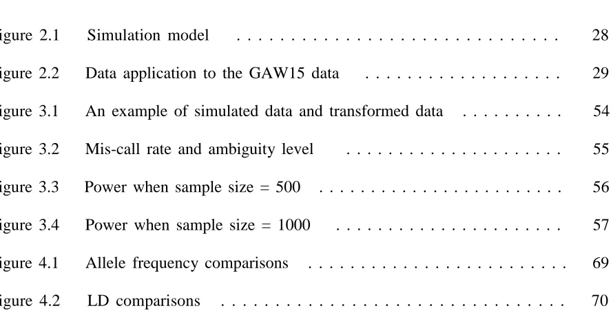
List of Figures

Figure 2.1 Simulation model . . . 28

Figure 2.2 Data application to the GAW15 data . . . 29

Figure 3.1 An example of simulated data and transformed data . . . 54

Figure 3.2 Mis-call rate and ambiguity level . . . 55

Figure 3.3 Power when sample size = 500 . . . 56

Figure 3.4 Power when sample size = 1000 . . . 57

Figure 4.1 Allele frequency comparisons . . . 69

(10)

Chapter 1

(11)

1.1 General introduction for association studies

Genetic association studies aim to detect association between the disease phenotypes and genetic polymorphisms. More and more attention has been focused on association analysis due to the rapid development of high-throughput genotyping technology, the availability of large amount of genetic marker and the completion of the initial wave of genetic maps (Neale 2004). During the past decade, association studies have been a promising tool to identify candidate genes or genomic regions that contribute to diseases. Causal genes for diseases, such as type I and type II diabetes, prostate cancer, breast cancer and inflammatory bowel diseases, have been found through genetic association studies (McCarthy 2008). These studies helped us to better understand the molecular mechanisms of diseases and will improve the medicine development in the future.

There are many different genetic markers that can be used to capture the genetic variation, such as restriction fragment length polymorphisms (RFLP’s), microsatellites, single

nucleotide polymorphisms (SNPs), and copy number variation (CNV). Among all the genetic markers, SNP is the most widely used one for human genetic disease mapping due to their high abundance across the human genome and the rapidly developed genotyping technology, although all the other genetic markers are still very important for genetic association research.

(12)

causal role; 2) indirect association, which means that the marker has no causal role but is associated with a nearby causal marker; and 3) confounded association, which is due to the population structure. Direct association is the easiest for association analysis and usually achieves the greatest power. Compared with the direct association, indirect association is much more difficult to detect and it is usually necessary to genotype more surrounding markers to pick up the causal marker. Population structure could result in false positive signals in association studies. To deal with confounded association, there are three strategies: matching by family, excluding population structure associated markers and using genomic control.

Based on how the samples are collected, association tests can be separated into two groups: population-based association test and family-based association test. Population-based analysis requires samples to be collected independently. The rational for population-based analysis is that the allele frequency distributions of the functional loci are different between cases and controls (Risch 2000). As we discussed in the previous paragraph, population structure is the main limitation of population-based test. The advantage of family-based test is that it is still valid even there was population structure. However, family data usually requires more resources in terms of money and time to collect data (Laird and Lange 2006). In the following discussion, we will only focus on population based association test.

(13)

most simple and natural association test is the single SNP based test. In the single SNP based test, the SNP was considered as the basic unit for testing. However, single SNP analyzing probably will neglect information due to joint effect of multiple SNPs. With increasing marker density, association is now often considered at the multiple marker level or haplotype level. Multiple SNPs based test can be used for testing the association between a gene and the phenotype given those SNPs are subject to an LD block within a gene. But the multiple SNP analysis can suffer from several problems: 1) too many parameters are needed to cover all the SNPs; 2) some of those SNPs are highly correlated. Another popular strategy

suggested by the block-like structure of the human genome is to use haplotype to capture the correlation structure of SNPs in regions of little recombination. Haplotypes can capture the combined effects of tightly linked cis-acting causal variants.

Despite the rapid improvement of genetic association analysis to date, there are still many limitations in methodologies. Here, we will focus on three problems which still exist in association test: how to incorporate covariates in haplotype similarity based test, how to avoid the power reduction induced by genotyping error, and how to improve the efficiency of large scale data simulation.

1.2 Haplotype similarity based association test

(14)

haplotype-based association tests have greater power when SNPs are in strong linkage disequilibrium with the disease locus (Akey 2001, Nielsen 2004, Zaitlen 2007) and are helpful in identifying rare causal variants (HapMap 2003, de Bakker 2005). However, the large dimensionality of haplotypes often leads to high degrees of freedom and the existence of rare haplotypes results in power loss in haplotype-based analyses (Seltman 2001, Molitor 2003(a), Thomas 2003, Zhang 2003, Durrant 2004, Sha 2005, Tzeng 2005, Yu 2005, Browning 2006).

To tackle the haplotype dimensionality problem, many methods have been proposed: (a) haplotype clustering (Seltman 2001, Molitor 2003(a), Durrant 2004, Tzeng 2005, Seltman 2003, Molitor 2003(b), Tzeng 2006), which clusters evolutionarily close haplotypes into groups, (b) haplotype smoothing (Molitor 2003(b), Thomas 2001, Schaid 2004), which smoothes haplotype effects by introducing a correlation structure on the effects of similar haplotypes, and (c) haplotype similarity (Houwen 1994, McPeek 1999, Su 2008), which looks for unusual sharing of chromosomal segments within homogeneous trait groups.

The general rationale behind the similarity method is that the haplotypes around a causative locus will be more similar among the cases descended from the common ancestors.

(15)

However, neither of the existing haplotype-similarity approaches can incorporate covariate information into analysis. This makes them less attractive for studying complex traits where covariate adjustments can be crucial. In chapter 2, we proposed an approach that combines the two schools of similarity approaches and is easy to incorporate covariates.

1.3 Genotyping error

High-throughput genome-wide SNP genotyping assay across many thousands of samples is required for association mapping study. It is important to notice that the performance of the genetic association methods depends on the novel high-fidelity genotyping technology and the accurate genotype determination. Many whole genome scan SNP chips have been developed recently, such as Illumina BeadArray, Affymatrix, Perlegen, and Tagman. Although genotyping technology has been considerably improved recently, further improvements are still necessary.

Many genotyping scoring algorithms have been published. Those genotyping scoring algorithms can be divided into two groups: (a) classification based method, and (b)

(16)

distribution, t mixture distribution or gamma distribution and the genotype can be determined by the probability of likelihood (Moorhead 2006, Xiao 2007, Teo 2007, WTCCC 2007).

Genotyping error is defined as the proportion of mistyping in all called genotypes.

Genotyping error includes the technological error and the scoring error (Kang 2004). Those technological problems have been improved during the recent years due to the technological development of genotyping whereas the scoring error is still a considerable problem.

Genotyping error could result in (1) incorrect estimates of allele frequency, linkage disequilibrium, genetic distance and (2) less power of association studies and linkage analysis (Goldstein 1997, Abecasis 2001, Akey 2001, Gordon 2002, Kang 2004, Hao 2004, Ahn 2006).

It is difficult to avoid genotyping scoring error under traditional association strategy. Recently, a couple of papers have been published that tried to incorporate genotyping uncertainty in association tests (Kang 2004, Zhu 2006). They used genotype probabilistic scoring instead of genotype as input to assess the association analysis. Simulation studies show that their methods can reduce the impact induced by genotyping errors because genotype probabilistic data provides more quantitative information. These two papers

(17)

1.4 Software for simulation

One key issue for developing novel association test is how to evaluate the power of each method under realistic settings. Simulation is an efficient way to evaluate the ability of novel methods to detect the disease markers. There are three main approaches for simulation (Liu 2008): 1) “backwards”, which starts with the samples that will form your simulated dataset, then works backwards in time to construct the genealogical information; 2) “forwards”, which starts with the entire population of individuals and then follows how all the genetic data are passed on from one generation to the next; 3) “Sidewards”, which starts with a collection of real genetic data, and uses these as a template for generating new simulated data with similar properties.

With the steady increase in public-available genomewide SNP data, such as the HapMap project, the potential advantage of the “sidewards” simulation approach has been realized recently. HapMap project, as a natural extension of the Human Genome Project, accelerates the pace of biomedical research. By providing abundant human genomic information, such as population information, LD block estimation, and accurate haplotype determination,

(18)

Chapter 2

A regression-based association test using inferred

ancestral haplotype similarity

Youfang Liu, Yi-Ju Li , Glen A. Satten, Andrew S. Allen and

(19)

2.1 Abstract

Objective: We propose a new association method based on haplotype similarity that incorporates covariates and utilizes maximum amount data information.

Methods: We first estimate the ancestral haplotypes of case individual and then, for each individual, an ancestral haplotype based similarity score is computed by comparing that individual’s observed genotype with the estimated ancestral haplotypes. Trait values are then regressed onto the similarity scores. Covariates can easily be incorporated under the

regression framework. To minimize the bias of raw p-values due to variation in ancestral haplotype estimation, a permutation procedure is adopted to obtain empirical p-values.

(20)

2.2 Introduction

Association analysis is becoming a primary approach for localizing disease loci, especially for detecting genes with modest effects on a disease. To access the association between genetic variants and disease, one can either consider individual SNPs or the haplotypes of closely linked SNPs. Although studies of their relative efficiency revealed varying

conclusions, it is generally appreciated that haplotype-based analyses have greater power when SNPs are in strong multilocus linkage disequilibrium with the disease locus (Akey 2001, Neilsen 2004, Zaitlen 2007), and are helpful in identifying rare causal variants (HapMap 2003, de Bakker 2005). However, practical potential of haplotype-based analysis may not be fully realized due to the difficulties balancing the dimensionality of the

haplotypes and the amount of information (Seltman 2001, Molitor 2003(a), Thomas 2003, Zhang 2003, Durrant 2004, Sha 2005, Tzeng 2005, Yu 2005, Browning 2006). The large dimensionality often leads to high degrees of freedom and the existence of rare haplotypes results in power loss in haplotype-based analyses.

(21)

McPeek 1999, Su 2008), which looks for unusual sharing of chromosomal segments within homogeneous trait groups. In this study, we focus on the haplotype-similarity approach, and introduce a method that aims to combine the merits of current similarity methods and incorporate covariate information.

Haplotype similarity methods have been constructed for association testing or for LD mapping. The general rationale behind the similarity method is that haplotypes around a causative locus will be more similar among cases descended from the common ancestors. Depending on how this concept is implemented, similarity methods can be divided into two categories: evolutionary based approaches and two-sample based approaches. Evolutionary based approaches tend to apply to cases only and the excess similarity among cases is identified by comparing to the similarity level expected from the genealogical process (Durham 1997, Service 1999). It takes direct advantage of the decay process of haplotype sharing, which is the underlying driving mechanism for haplotype similarity (McPeek 1999, Su 2008, Morris 2002, Morris 2003, Morris 2005). However, it becomes more challenging to model the genealogical process for complex diseases because the causal variants have a relatively modest impact on total disease risk (Zöllner 2005).

(22)

concordant samples (i.e., case-case similarity and control-control similarity). Further, many of these methods do not use information obtained from case-control similarity. Sha et al. (2007) showed that by accounting for the information from discordant pairs, the power of using haplotype similarity to detect association is significantly improved (Sha 2007). Finally, the existing haplotype-similarity methods do not incorporate covariate information. This makes them less attractive for studying complex traits where covariate adjustments can be crucial.

In this article, we propose an approach that combines the two schools of similarity

approaches to addresses current concerns. Our method follows the framework of two-sample approaches, while the level of similarity in each sample is quantified following the spirit of evolutionary-based approaches. Specifically we estimate the ancestral haplotypes of cases using the multilocus decay-of-haplotype-sharing (DHS) model of McPeek and Strahs (1999), and use the estimated ancestral haplotypes as the “summary haplotypes” of the case

haplotypes. We then define the “ancestral haplotype similarity (AHS) scores”, which

(23)

of the case haplotypes, we bypass the issue of whether the estimated ancestral haplotypes are actually the true ancestral disease haplotypes for complex traits.

In the following sections, we illustrate the procedure of the proposed AHS method, and present simulation results of type I errors and power. The results are compared to the standard haplotype score test of Schaid et al. (2002). We also applied our method to the simulated SNP data for Rheumatoid Arthritis (RA) from GAW (Genetic Analysis Workshop) 15 and examined whether this proposed method can detect the DR and D loci that affect the risk of RA.

2.3 Methods

2.3.1 Model and approach

(24)

account for the estimation error induced from the use of the estimated ancestral haplotypes. Below we describe each of the steps in detail.

In the first step, we use the DHS method (McPeek 1999, Strahs 2003) to infer the ancestral case haplotypes. The DHS method models the decay process of haplotype sharing for haplotypes descended from certain common ancestors, taking into account recombination, mutation, and background LD. The model allows for multiple origins of case haplotypes, and incorporates haplotype correlation due to shared ancestry by applying a correction factor to the star-shaped genealogy of case haplotypes. The method has been implemented in the software of DHSMAP (Decay of Haplotype Sharing Mapping), and can take phased haplotypes (McPeek 1999) or unphased genotype data (Strahs 2003).

(25)

the count of the matching alleles between the genotype of individual i and ancestral

haplotype j. The weight for ancestral haplotype j is _j j

k k

L w

L

=

∑

, k is the number of all inferred

ancestral haplotypes, and the overall AHS score for person i is _i ij j

j

S =

∑

s w .

In the third step of evaluating association between haplotypes and disease status, we fit a

generalized linear model (McCullagh 1989):g

( )

µi =γtXi+βSi, where Xi is the design

matrix of covariates including the intercept , g

( )

⋅ is the link function, and µ_i =E Y X S

(

_i| _i, _i

)

with Y_i equaling to the trait value. The null hypothesis of no association corresponds to β = 0.

To address the extra variability introduced into the procedure by using estimated ancestral haplotypes, we use permutation procedure to obtain the empirical p-values. The permutation datasets are obtained by randomly shuffling individual’s genotype instead of phenotype, so to maintain the potential association between the phenotype and the covariates. For each

permutated dataset, we repeated the entire procedure of estimating the ancestral haplotypes, computing similarity scores and fitting the regression model. Empirical p-values were computed as the proportion of significant results from all the permutation datasets. All analysis procedures were implemented using R software (http://www.r-project.org/).

2.3.2 Simulation study

(26)

thirty trio families in the original CEU data set. To create an unrelated random population, we selected two parents from each family to form a sample pool and randomly drew cases and controls from this pool with replacement. We focus on the shortest chromosome 22 to facilitate data processing.

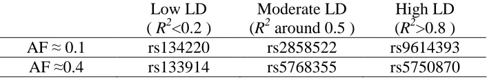
We consider six simulation scenarios, as listed in Table 2.1, with different allele frequency (AF) of the causal variant (0.1 and 0.4) and different LD between the causal variant and its

surrounding LD (high (R2 >0.8), moderate (R2 ≈0.5) and low (R2<0.2)) (Table 2.1). For each scenario of AF and LD, a SNP was chosen as the causal locus in accordance with the simulation setting. Given a causal locus, the three neighboring markers (one marker to its left and two to its right) form a haplotype of size 3 (Figure 2.1). We then randomly draw two haplotypes with replacement and convert it to the unphased genotype for an individual. Therefore, the observed genotype of an individual does not include the causal locus, though the trait value is determined by the genotype of the causal marker using the logistic model:

Logit [ Pr ( Y=1 | G, E ) ] = γ0+ × +γ1 E βg×G, where Y is the disease status coded as 0 and

(27)

logistic model parameters were set asγ₁=1.0 and γ₀ = −4 which corresponds the population

prevalence rate of 0.03. For type I error analysis, β was set to be log(1.0), and for power analysis, βg = log(1.5). We obtained the empirical p-value by 104 permutations.

2.3.3 Data application to GAW15 data

The Genetic Analysis Workshop (GAW) has provided several sets of data biannually since 1982. In 2006, GAW15 provided the simulated Rheumatoid Arthritis (RA) SNP data which includes the HLA DR locus and the D locus on chromosome 6. The DR locus directly affects risk of RA while D locus increases RA risk 5-fold. According to the simulation

information provided by GAW, smoking status is a very important covariate which can affect RA risk directly.

We selected one child from each affected sib-pair family to create a case pool. We randomly selected N individuals from this case pool and N controls from all the controls in the

(28)

2.4 Results

2.4.1 Simulation study

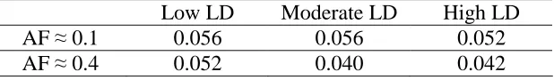
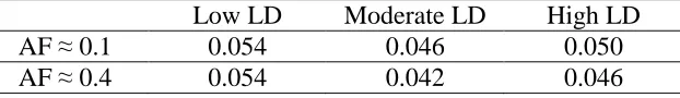
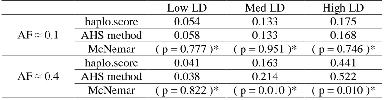
Table 2.2 and Table 2.3 displays the type I error of the AHS tests which was calculated on the basis of 1000 simulation replicates for 200 samples and 400 samples respectively. The values in Table 2.2 and Table 2.3 are close to the nominal level 0.05, indicating that the type I error is under controlled. Table 2.4 and Table 2.5 show the power at the nominal level 0.05 obtained on the basis of 500 simulation replicates for 200 samples and 400 samples

respectively. The power of the AHS method is compared to the standard haplotype score test of Schaid et al. (2002) as implemented in the R function haplo.score. We also performed a McNemar test to examine whether the power difference is significant. First, as expected, when the disease locus in low LD with its nearby markers, there is no statistical power to detect the association for both of the method, and hence the power is around the nominal level. When the disease locus is in moderate or high LD with surrounding SNPs, we notice that the power performance depends on the disease allele frequency. The power of the two methods is not significantly different when the disease allele frequency is low. When the disease allele frequency is high, the power of AHS method is significantly higher than the standard haplotype method.

2.4.2 Data application to the GAW15 data

(29)

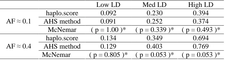
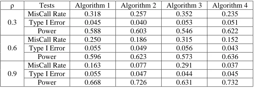
the profile of empirical p-values over chromosomal locations. The peak of empirical p-values is surrounding 49.45cM where the true causal HLA DR locus lies. We also plotted p-values from haplo.score test in Figure 2.2a. It clearly shows that both methods are capable of detecting the disease causal signal.

Under the 400 samples situation, The AHS method identified two very close regions (Figure 2.2b). One region is exactly the same region as described above. The other one is a 1cM region containing 8SNPs and being highly linked with the first region.

On the other hand, both methods did not detect the second disease loci, the D locus located 5.12cM downstream from the DR locus on chromosome 6 whenever 200 samples or 400 samples were used for analysis.

2.5 Discussions

In this work, we proposed a new haplotype similarity method that is under the regression framework and uses the ancestral haplotype similarity scores, which are obtained by comparing individual haplotypes with the inferred ancestral haplotypes of the cases. Using the ancestral haplotypes as a reference for scoring similarity provides a possible mechanism to tackle several common issues encountered in current similarity-based approaches,

(30)

haplotypes, we assign an AHS score to each individual. Through the AHS scores, the traditional similarity comparison between two samples (case-case pairs vs. control-control pairs or concordant pairs vs. discordant pairs) is now transformed to testing the association between the trait values and the AHS scores. With this transformation, the haplotype similarity information of each sample is retained and used, and the association can be examined naturally under a regression model so to account for covariates and various trait types. Finally, we define the similarity score based on the number of matching alleles

between compared haplotypes, which allows for un-phased genotypes and avoids estimation of the haplotype phase for each individual.

As a quick note, we would like to point out that besides using AHS scores as proposed here, there also exist alternative approaches to tackle the common issues mentioned above in the similarity-based approaches, such as Tzeng et al. (2008). In these approaches, the use of the pairwise samples is extended to a model-based framework, and the focus is to study the correlation between the trait similarity and haplotype similarity. It may be interested to understand the relative efficacy of method of this type and the AHS methods.

(31)

the estimated ancestral haplotypes be representative of the case haplotypes, so that the similarity scores of each individual reflect similarity to case haplotypes. For the latter concern, we chose to perform permutation tests. In our permutation, we choose to permute the genetic information instead of the disease status among individuals. Such procedure retains the relationship between the disease status and the potential covariates.

(32)

Tables

Table 2.1 The six simulation scenarios for causal locus Low LD

( R2<0.2 )

Moderate LD (R2 around 0.5 )

High LD (R2>0.8 ) AF ≈ 0.1 rs134220 rs2858522 rs9614393

(33)

Table 2.2 Type I error at nominal level 0.05 (100 cases and 100 controls) Low LD Moderate LD High LD

AF ≈ 0.1 0.056 0.056 0.052

(34)

Table 2.3 Type I error at nominal level 0.05 (200cases and 200 controls) Low LD Moderate LD High LD

AF ≈ 0.1 0.054 0.046 0.050

(35)

Table 2.4 Power at nominal level 0.05 (100 cases and 100 controls)

Low LD Med LD High LD

haplo.score 0.054 0.133 0.175

AHS method 0.058 0.133 0.168

AF ≈ 0.1

McNemar ( p = 0.777 )* ( p = 0.951 )* ( p = 0.746 )*

haplo.score 0.041 0.163 0.441

AHS method 0.038 0.214 0.522

AF ≈ 0.4

(36)

Table 2.5 Power at nominal level 0.05 (200 cases and 200 controls)

Low LD Med LD High LD

haplo.score 0.092 0.230 0.394

AHS method 0.091 0.252 0.374

AF ≈ 0.1

McNemar ( p = 1.00 )* ( p = 0.339 )* ( p = 0.493 )*

haplo.score 0.134 0.349 0.694

AHS method 0.129 0.403 0.769

AF ≈ 0.4

(37)

Figures

Figure 2.1 Simulation model

(38)

0 2 4 6 8 1 0

(a) Sample Size = 200

cM -l o g 1 0 (p -v a lu e s )

48 DR 50 52 54 D 56

0 2 4 6 8 1 0

(b) Sample Size = 400

cM -l o g 1 0 (p -v a lu e s )

48 DR 50 52 54 D 56

Figure 2.2 Data application to the GAW15 data

(39)

Chapter 3

Association Studies Using Intensity Data

(40)

3.1 Abstract

Current genotyping technology produces two dimensional intensity data, from which

genotypes are inferred by a scoring algorithm and genetic association are evaluated based on the scored genotypes and phenotypes. Genotyping scoring errors remain a major challenge for automated scoring programs and it renders a negative impact on association analysis. Here, we propose an alternative strategy that uses the intensity data to study gene-trait association. In the analysis, we treat the original two dimensional intensity data or their transformation as the observed genetic variables and regard genotypes as unobserved variables. The genotyping uncertainty is hence incorporated in the assessment of the

association. Simulation studies demonstrate that intensity information based association test slightly outperforms other approaches that use inferred genotypes as input when mis-call rate is high.

3.2 Introduction

SNPs, single nuclear polymorphism, the most abundant and stable marker, are widely used in linkage analysis, association mapping and complex disease study (Risch 2000). With the completion of the Human Genome Project, a huge volume of SNPs have been discovered in the human genome (The international HapMap consortium 2005). With more SNPs

(41)

genome (Gabriel 2002, Judson 2002, Stephens 2001). Therefore, high-throughput genome-wide SNP genotyping assay across many thousands of samples is required for association mapping study, and the performance of the abovementioned association studies depends on the high-fidelity genotyping technology.

Genotyping can be separated into two steps: allele discrimination and allele detection. Allele discrimination is the generation of specific products for SNPs, which is done by allele-specific biochemical reaction (Syvanen 2001, Kim 2007). There are four different allele discrimination methods: enzymatic cleavage, hybridization with allele-specific probes, oligonucleotide ligation, and single primer extension (Syvanen 2001, kim 2007). Allele detection methods include indirect colorimetric, chemiluminescence, fluorescence, fluorescence resonance energy transfer, fluorescence polarization, mass spectrometry (Syvanen 2001, Kim 2007). Many whole genome scan SNP chips have been developed recently, such as Illumina BeadArray, Affymatrix, Perlegen, and Tagman, etc. They use different allele discrimination methods and allele detection methods (Syvanen 2001). For example, the TagMan assay involves hybridization with allele specific probes and detection by fluorescence resonance energy transfer (Syvanen 2001). Although genotyping technology has been considerably improved recently, further improvements are still necessary in order to improve the quality and efficiency of genotyping (Syvanen 2001, Kim 2007).

(42)

2002, Liu 2003, Rabbee 2006, Bierut 2007), and (b) distribution based method (Fujisawa 2004, Di 2005, Hua 2006, Nicolae 2006, Moorhead 2006, Xiao 2007, Teo 2007, WTCCC 2007). Among the recently published classification based methods. Oliver’s method and Bierut’s method are both based on the K-means clustering strategy (Oliver 2002, Bierut 2007). Liu et al. proposed the modified partitioning around medoids as a classification method for relative allele signals (Liu 2003). RLMM (Rabbee 2006) and BRLMM (Cawley 2006) are very similar and both based on a robustly fitted linear model and use the

(43)

a newly developed algorithm for Affymetrix SNP chip data, is based on a Bayesian hierarchical mixture model and is one of the scoring algorithms used for WTCCC project.

For genetic association analysis, the major concern is the genotyping error. It could result in incorrect estimates of allele frequency, linkage disequilibrium, and genetic distance. It can also reduce the power and increase the false positives of association analysis (Goldstein 1997, Abecasis 2001, Akey 2001, Gordon 2002, Kang 2004, Hao 2004, Ahn 2006).Genotyping error is defined as the proportion of mistyping in all called genotypes that can be categorized into two groups: the technological error and the scoring error (Kang 2004). Those

technological problems have been addressed in recent years by the improvement of genotyping technology whereas the scoring error is still a considerable problem.

(44)

genotype before doing the haplotype inference. They found that probabilistic scoring gives rise to more quantitative information and flexibility in the haplotype phasing step and can improve the accuracy in haplotype phasing, especially in high LD and high ambiguity situation (Kang 2004). Zhu moved one step further: they not only estimated possible

genotypes thus the haplotype inference but also did the haplotype association test (Zhu 2006). Simulation studies show that their likelihood-based method reduced the impact by

genotyping errors. These two papers discussed above are focusing on haplotype inference and haplotype association test. The similar principle can be applied to SNP-based analysis.

Here, we propose an algorithm that incorporates the genotyping uncertainty to assess the association between trait data and SNPs. In this strategy, we use the original two-dimensional intensity data or the transformed one-dimensional intensity data as input and regard

genotypes as unobserved variables. We also considered alternatively strategies that are commonly used in practice to reach a better understanding on how different strategies would optimally be applied to various scenarios.

3.3 Methods

3.3.1 Transformation algorithms of the two-dimensional intensity data

(45)

Algorithm 1 (Cawley 2006): X = asinh[ 4 ( Ia– Ib ) / ( Ia + Ib ) ] / asinh( 4 ),

Algorithm 2 (Teo 2007): X = ( Ia - Ib ) / ( Ia + Ib ),

Algorithm 3 (Bierut 2007): X = Ia / ( Ia + Ib ),

Algorithm 4 (Moorhead 2006): X = sinh[ 2 ( Ia– Ib ) / ( Ia + Ib ) ] / sinh( 2 ),

* sinh(m)=(exp(m)-exp(-m))/2.

In the algorithms above, Ia stands for probe intensity of allele “a” and Ib stands for probe

intensity of another allele “A”. After transformation, X follows a normal distribution, N(μg,σg2), with g stands for three different genotypes AA, Aa, and aa.

Many scoring algorithms have been proposed in recent years. In this work we particularly focus on the genotype determination algorithm of Moorhead et al. (2006). The algorithm firstly transforms the two dimensional intensity data into one dimensional data using Algorithm 4 and then fit the transformed data using a mixture normal distribution. It estimates the parameters by EM algorithm, and determines the genotype based on the likelihood value. We choose Moorhead’s method because it is easier to write the likelihood for one dimension data and it is easy to achieve convergence for EM algorithm when there is less parameter in the model.

3.3.2 Likelihood of the complete data

The observed data are the original or transformed intensity data (denoted by R),

(46)

follows, from which we can use EM algorithm to obtain MLEs of the observed-data likelihood or the score function of the observed-data likelihood:

(1) L = f (Y, G, R | E ) = f ( Y | G, R, E ) f ( G, R ) = f ( Y | G, E ) f ( G, R ), where Y is the trait data, R is the input data which could be the original two dimensional intensity data or the transformed one dimensional data, G is genotype ( AA = 0, Aa = 1, aa = 2 ) and E is the covariate;

(2) f ( G, R ) = mixture of normal distribution, which will be discussed in the next paragraph; (3) f ( Y | G, E ) = exp{ ( Yη– b ( η ) ) / a ( φ ) + c ( Y, φ ) }, which is expressed as an exponential family data, where a, b and c are known functions, φ is the dispersion parameter and η is the link function;

(4) η = β0 + βgG + βeE, where β0,βg and βe are the regression parameters for the intercept, the

genotype factor and environmental factor, respectively.

We fit two different normal mixture models for f ( G, R ) : (1) univariate normal mixture distribution model, which uses transformed data X of Algorithm 4 as input data; and (2) bivariate normal mixture distribution, which uses original two dimensional probe intensity data Ia and Ib as input. For the i-th sample, we can write its un-normalized probability of

belonging to the j-th cluster, with respect to the two normal mixture models abovementioned, as follows:

(1) fij ( G = j, Ri = Xi ) = ( λj / σj ) exp ( -1/2 ( ( Xi - mj ) / σj )2 ), where mj, σj and λj are the

(47)

(2) fij ( G = j, Ri = ( Iai, Ibi ) ) = ( λj / ( σxjσyj ( 1 - ρ2 )1/2 ) ) exp { -1 / ( 2 ( 1 - ρ2 ) ) [ ( Iai -

mxj )2 / σxj2 + ( Ibi - mxj )2 / σxj2 + ( Iai - mxj ) ( Ibi- myj ) / ( σxjσyj ) ]}, where mxj, myj, σxj, σyj, ρj

and λj are the mean, sigma, and weight of the jth cluster, respectively.

3.3.3 Score test for H0: βg = 0

Let θ =

(

β ψg,

)

, where βg is of our interest and ψ =

(

β β φ φ φ0, e, 0, ,1 2

)

is the nuisance

parameter. In the one-dimensional intensity based score test approach, we define

(

, ,

)

0,1, 2

j j j j j

φ = µ σ λ ∀ = for each genotype cluster. In the two-dimensional intensity

based score test, we have φ_j =

(

µ µ σ σ ρ λ_xj, _yj, _xj, _yj, _j, _j

)

∀ =j 0,1, 2.

We are interested in testing the hypothesis H0:βg =0. Denote ψ% as the maximum

(48)

( )

(

)

(

)

( )

0, 2 2 log , log 0, 0, 0, and

0, log 0, log ,

0, where log 0, , log 0, g g g g g

g g g g g g g g g g L L S S

S L L

I I I I I L I E L I E β ψ β ψ ψ β β β ψ ψβ ψψ β β β ψ β ψ ψ ψ β β ψ ψ ψ _{β ψ} ψ _ψ ψ ψ β β = = ∂   ∂        _ ∂ _ _ ∂ _ =_ _=_ _=_ _ ∂ _∂   _ _    _∂ _{ } _   _ ∂ _     = _ _  ∂  = _− _ ∂ ∂     ∂ = − % % % % % % % %

( )

2 , log 0, . g L

I_ψψ E

ψ β ψ ψ ψ ψ    _{∂ ∂}       ∂  = _− _ ∂ ∂   % %

Next we use Louis’s method (Louis 1982) to compute the score statistic of the observed likelihood (note the asterisks that denote statistics for observed data) as follows:

( )

* * 1 *

0, 0,

g g g

T_β =S_β ψ% V S− _β ψ%

where *

( )

0,

( )

0,

g g

S_β ψ% = E S _β ψ% _ and

( )

1

( )

* * * * *

var 0, 0, 0, 0, 0,

g g g g g

V = _S_β ψ% _=I_{β β} ψ% −I_{β ψ} ψ% _I_ψψ ψ% _− I_ψβ ψ% .

In the above equations,

( )

*

0, 0, ,

S ψ% = E S_ ψ% _ I*

( )

0,ψ% =E I_

( )

0,ψ% _−E S_

( ) ( )

0,ψ% ST 0,ψ% _+S*

( ) ( )

0,ψ% S* 0,ψ% . Note that *

( )

0,

g g

(49)

3.3.4 Five strategies for testing association

We will discuss five different association tests using either genotype or intensity data as input.

Test 1: Score test using true genotypes. Test 2: Score test using estimated genotype

Test 3: Score test using estimated genotype probability

Test 4: Score test using the one dimensional transformed intensity data Test 5: Score test using the two dimensional original intensity data

3.3.5 Simulation schemes

To compare the performance of using intensity data with that of using genotypes, we

simulated probe intensity data for each SNP such that each genotype cluster’s shape and size are similar to that of the real probe intensity data. We assumed Hardy-Weinberg equilibrium (HWE) for each SNP in the simulated population and multivariate t distribution for each cluster of genotype. Each of the three different genotypes has a multivariate t distribution with different mean and variance matrix. Each genotype cluster has a center and spreads in two dimensions with a constant variance. The ambiguity level is controlled by changing the correlation coefficient ρ, the correlation coefficient of the variance matrix. Many scenarios were simulated with different ρ, allele frequencies and sample sizes. Detailed simulation procedure is as follow:

(50)

2. Simulate the two dimension probe intensity data using a multivariate t distribution. 3. Determine the disease status for each individual based on the logistic regression model: Logit [ Pr ( Y=1 | G, E ) ] = β0 + βgG + βeE.

4. Repeat step 1, 2, and 3 until obtaining enough cases and controls. Two different sample size, 500 and 1000, were set to illustrate how sample size will affect power.

5. Generate 1000 replicates for power and type I error analysis.

3.3.6 Application to the WTCCC data

In 2007, the Wellcome Trust Case Control Consortium (WTCCC) provided several data sets including one control data set from the 1958 UK Birth Cohort, another control data from the UK National Blood Service and case data sets for seven diseases, such as Type 1 diabetes, Type 2 diabetes, rheumatoid arthritis, inflammatory bowel disease, bipolar disorder,

(51)

3.4 Results

3.4.1 Comparisons of the four different transformation algorithms

We compared the performance of four different transformation algorithms described in methods under different ambiguity levels from low to high. In our simulation, bivariate t

distributions were used to generate the fluorescence intensity (FI) scatter plots (see Figure 3.1 shows an example of simulated two dimensional intensity data). We determined the genotype for each individual through Moorhead’s method and calculate the miscall rate for each transformation algorithm. We also performed the SNP single marker association test with genotype uncertainty based on four different transformed data and calculated the power.

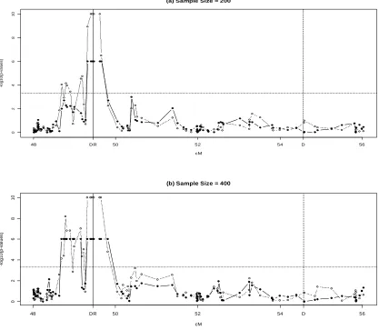
Table 3.1 shows miscall rates for all the transformation algorithms under different ambiguity level. To make a fair comparison, we gave the same starting points for the centroids for all the algorithms. In the mixed normal model, we picked the cluster with the highest probability. We counted the number of erroneous calls (defined as the calls different from the true calls) in each simulation scenario. At every ambiguity level, the Algorithm 4 outperformed other algorithms.

(52)

3.4.2 Ambiguity level and mis-call rate

The ambiguity level of the two dimension intensity data is controlled by changing the correlation coefficient for the covariates matrix, ρ, which is also called the ambiguity parameter. Mis-call rate is the percentage of the mis-classified genotypes among all the genotypes. To describe the relationship between ρ and call rate, we calculated the mis-call rates based on five different ρ values ranging from 0.1 to 0.9. As the ambiguity

parameter increases, the mis-call rate decreases (Figure 3.2).

3.4.3 Power comparisons of different association tests

To find which association test performs better, we compared different association tests under many scenarios with different sample sizes, allele frequencies and ambiguity levels. A thousand replicates under each scenario were simulated for type I error and power analyses.

Table 3.2 and Table 3.3 show the type I errors for all the association test methods with sample sizes of 500 and 1000, respectively. All the type I errors are close to the nominal level of 0.05, which verifies the validity of the test statistics constructed here.

(53)

transformed intensity based test and two dimensional intensity based test yielded similar power. When ambiguity level increases, transformed one-dimensional intensity based test has the highest power among all the methods.

We set four different minor allele frequencies at 0.01, 0.05, 0.10 and 0.25. The power trends for all the allele frequencies are similar. We noticed that it is very difficult for two

dimensional intensity based test to estimate the centroid and variance of the minor allele homozygote genotype group when sample size is equal to 500 and minor allele frequency is lower than 0.1. After increasing the sample size to 1000, two dimensional intensity based test obtained the ability to handle simulated data with allele frequency 0.05. Thus, with enough sample size, such as 5000 or more, two dimensional intensity based test would possibly overcome the problem for small sample size and low allele frequency.

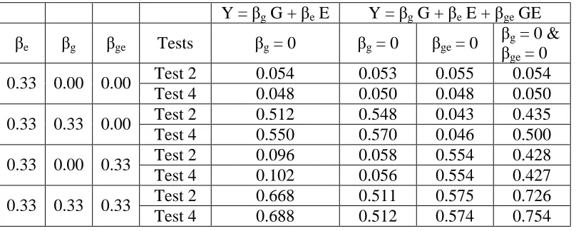
3.4.4 Gene-Environment interaction

Increased attention has been paid on gene-environment interaction for complex disease association study. The above framework can be extended to incorporate the gene-environmental interaction:

Y = β0+G + βeE + βgeGE,

where Y stands for the trait, G for the genotype, E for the environment effect, and GE for the interaction term. We tested the genetic effect βg = 0, interaction effect βge = 0, and combined

(54)

to 500, set the ambiguity parameter at 0.7 and the allele frequency to 0.25. The results for four different scenarios are in the Table 3.4 and discussions are as follows:

(1) βe = log(1.4), βg = log(1.0), βge = log(1.0). Under this null scenario, there is no genetic

effect and no gene-environment interaction effect. All the tests successfully controlled their type I errors around the nominal level of 0.05.

(2) βe = log(1.4), βg = log(1.4), βge = log(1.0). Since this is the genetic effect only scenario, it

is reasonable that we couldn’t detect the power by testing βge alone. The simulation results

demonstrated that intensity based method outperformed the genotype based method when testing βg effect alone or βg and βge combined.

(3) βe = log(1.4), βg = log(1.0), βge = log(1.4). Under this scenario, the model contains the

gene-interaction effect only. It is interesting to see that the performance of intensity based tests was very similar with that of genotype based test.

(4) βe = log(1.4), βg = log(1.4), βge = log(1.4). This is the most general scenario which

contains both the genetic effect and the interaction effect. When testing βg = 0 or βge = 0, both

testing methods obtained similar level of power. However, when testing βg and βge jointly, the

intensity based test outperformed the genotype based test.

3.4.5 Application to the WTCCC data

(55)

dimensional intensity data were available. We performed the intensity based test and the genotype based test, respectively. According to several association studies to date, there are totally nine susceptive genes and 11 causal loci for Type 2 Diabetes (Zeggini 2007).

However, two loci (rs1111875 and rs13266634) were missing from the WTCCC dataset and hence there were only eight susceptive genes and 9 causal loci included in our analysis. Genotype-based score test and intensity-based score test both identified all the 9 loci and eight susceptive genes. The results are summarized in Table 3.5 that also included the p-values from a previous association study (Zeggini 2007) using WTCCC data set with

different number of cases and controls. Comparing our results with the p-values provided by Zeggini’s paper, we found that both genotype-based test and intensity-based test got very similar p-values as the previous study.

3.5 Discussions

(56)

can reduce the impact by genotyping errors. To date, there is no published method using intensity data as input for SNP based association test. Single marker based association test is generally more widely used than haplotype test in genome-wide association studies due to its simplicity and computational efficiency. In this paper, we proposed a new score test that incorporates the genotyping uncertainty to assess the association between traits and SNPs. In this method, we directly used the original intensity data and regard genotypes as unobserved variables such that genotyping scoring errors would not be a problem. Our simulation studies showed that association analysis using intensity data can improve the power comparing to other approaches using inferred genotypes.

Poor separation between genotype clusters always increases the mis-call rate and thus impacts the association test. The results of power comparison in association test showed that all intensity based test (genotype probability based score test, one dimensional data based score test and two dimensional probe intensity data based score test) had power

improvements comparing with inferred genotype based score test when mis-call rate is high.

Two dimensional original intensity data is supposed to contain more quantitative information than transformed one dimensional data. It was surprising that one dimensional data based score test has higher power than two dimensional data based score test under almost all the simulation scenarios. One possible cause could be that two dimensional data based

(57)

which, during Expection-Maximization iterations, could make it more difficult to achieve the convergence.

Since the two dimensional intensity based score test faces the convergence problem in the EM algorithm, it is limited in sample size and allele frequency. When sample size is small and allele frequency is low, there will be few individuals with homozygous minor alleles. Under such situation, it is very difficult for EM algorithm to estimate its centroid and variance. Based on the reasons above, two dimensional intensity based score test can not be applied to a data set with small sample size and low allele frequency simultaneously. However, one dimensional intensity based score test has the ability to overcome the convergence problem encountered during the EM procedure.

(58)

Tables

Table 3.1 Comparing four different transformation algorithms

ρ Tests Algorithm 1 Algorithm 2 Algorithm 3 Algorithm 4

MisCall Rate 0.318 0.257 0.352 0.235

Type I Error 0.045 0.040 0.053 0.051

0.3

Power 0.588 0.603 0.546 0.622

MisCall Rate 0.250 0.186 0.315 0.152

Type I Error 0.055 0.049 0.056 0.043

0.6

Power 0.596 0.623 0.573 0.636

MisCall Rate 0.163 0.077 0.291 0.037

Type I Error 0.055 0.047 0.044 0.045

0.9

(59)

Table 3.2 Type I error when sample size = 500

AF ρ 0.9 0.7 0.5 0.3 0.1

MisCall Rate 0.008 0.082 0.147 0.193 0.227

Test 1 0.045 0.039 0.046 0.055 0.048

Test 2 0.044 0.040 0.054 0.054 0.052

Test 3 0.055 0.041 0.046 0.053 0.048

Test 4 0.055 0.041 0.048 0.055 0.047

0.01

Test 5 - - - - -

MisCall Rate 0.014 0.090 0.153 0.200 0.236

Test 1 0.048 0.049 0.050 0.044 0.047

Test 2 0.054 0.055 0.040 0.042 0.050

Test 3 0.052 0.054 0.045 0.052 0.045

Test 4 0.052 0.054 0.045 0.052 0.047

0.05

Test 5 - - - - -

MisCall Rate 0.020 0.098 0.162 0.210 0.245

Test 1 0.053 0.045 0.044 0.047 0.041

Test 2 0.051 0.052 0.049 0.042 0.051

Test 3 0.041 0.053 0.041 0.048 0.047

Test 4 0.044 0.053 0.036 0.039 0.048

0.10

Test 5 0.030 0.035 0.033 0.038 0.040

MisCall Rate 0.035 0.116 0.181 0.230 0.270

Test 1 0.052 0.043 0.052 0.050 0.047

Test 2 0.048 0.051 0.050 0.046 0.058

Test 3 0.046 0.043 0.045 0.049 0.047

Test 4 0.048 0.044 0.044 0.049 0.046

0.25

(60)

Table 3.3 Type I error when sample size = 1000

AF ρ 0.9 0.7 0.5 0.3 0.1

MisCall Rate 0.009 0.082 0.147 0.193 0.226

Test 1 0.052 0.048 0.055 0.040 0.050

Test 2 0.046 0.042 0.052 0.046 0.055

Test 3 0.040 0.045 0.054 0.040 0.054

Test 4 0.042 0.046 0.054 0.041 0.053

0.01

Test 5 - - - - -

MisCall Rate 0.016 0.091 0.155 0.202 0.239

Test 1 0.048 0.049 0.050 0.056 0.051

Test 2 0.052 0.047 0.048 0.042 0.048

Test 3 0.051 0.041 0.050 0.048 0.054

Test 4 0.048 0.041 0.052 0.048 0.054

0.05

Test 5 0.044 0.045 0.040 0.042 0.048

MisCall Rate 0.023 0.101 0.166 0.214 0.249

Test 1 0.047 0.055 0.056 0.048 0.055

Test 2 0.050 0.044 0.044 0.042 0.047

Test 3 0.052 0.052 0.044 0.051 0.053

Test 4 0.051 0.053 0.044 0.052 0.052

0.10

Test 5 0.040 0.039 0.049 0.038 0.040

MisCall Rate 0.035 0.116 0.182 0.231 0.268

Test 1 0.047 0.042 0.046 0.050 0.046

Test 2 0.050 0.049 0.051 0.054 0.043

Test 3 0.050 0.045 0.050 0.051 0.047

Test 4 0.051 0.044 0.051 0.050 0.046

0.250

Test 5 0.044 0.042 0.047 0.055 0.040

(61)

Table 3.4 Power for genetic model including gene-environment interaction Y = βg G + βe E Y = βg G + βe E + βge GE

βe βg βge Tests βg = 0 βg = 0 βge = 0 βg

= 0 &

βge = 0

Test 2 0.054 0.053 0.055 0.054

0.33 0.00 0.00

Test 4 0.048 0.050 0.048 0.050

Test 2 0.512 0.548 0.043 0.435

0.33 0.33 0.00

Test 4 0.550 0.570 0.046 0.500

Test 2 0.096 0.058 0.554 0.428

0.33 0.00 0.33

Test 4 0.102 0.056 0.554 0.427

Test 2 0.668 0.511 0.575 0.726

0.33 0.33 0.33

(62)

Table 3.5 Data application to the WTCCC data

Rs Chr Gene

p-values from previous

paper

Test 2 Test 4

Rs1801282 3 PPARG 1.3e-03 3.8e-04 1.1e-03

Rs4402960 3 IGF2BP2 1.7e-03 1.7e-03 7.9e-05 Rs10946398 6 CDKAL1 2.5e-05 1.6e-05 7.9e-06

Rs564398 9 CDKN2B 3.2e-04 8.3e-04 7.2e-03

Rs10811661 9 CDKN2B 7.6e-04 1.2e-03 5.4e-03

Rs5015480 10 HHEX 5.4e-06 2.4e-05 1.2e-06

Rs7901695 10 TCF7L2 6.7e-13 8.6e-14 4.9e-14

Rs5215 11 KCNJ11 1.3e-03 1.7e-03 5.3e-03

(63)

Figures

Figure 3.1 An example of simulated data and transformed data. a. The left one: plot for the two dimensional original data. b. The right one: histogram for the one dimensional transformed data.

Histogram of transformed data

all.trans F re q u e n c y

-0.5 0.0 0.5 1.0

0 5 1 0 1 5 2 0 2 5 3 0

0 2 4 6 8 10 12 14

0 5 1 0 1 5

Raw FI Data

Fluorescent Intensity For Allele a

(64)

0.0 0.2 0.4 0.6 0.8 1.0 0 .0 0 0 .0 5 0 .1 0 0 .1 5 0 .2 0 0 .2 5 0 .3 0

Rho: Ambiguous Parameter

M is C a ll R a te

0.0 0.2 0.4 0.6 0.8 1.0

0 .0 0 0 .0 5 0 .1 0 0 .1 5 0 .2 0 0 .2 5 0 .3 0

M is C a ll R a te

Figure 3.2 Mis-call rate and ambiguity level

(65)

0.9 0.7 0.5 0.3 0.1

AF = 0.01