ABSTRACT
CRILL, JOHN WESLEY. Ad-hoc Solutions for Capturing Electronic Structure Details in Classical Dynamics Simulations. (Under the direction of Prof. Donald W. Brenner. and Prof. Douglas L. Irving.)
Traditional empirical potentials used in molecular dynamics (MD) simulations replace an explicit treatment of the electronic structure with an appropriate interatomic potential energy expression. This enables MD simulations to model atomistic processes, such as dislocation dynamics and plastic deformation, which typically require size and time domains exceeding what is currently feasible with computationally-demanding first
principles techniques. However, discarding the electronic degrees of freedom prevents MD simulations from properly resolving certain phenomena which are dominated by electronic interactions. One example is thermal transport in metals, which is often underestimated by orders of magnitude in MD simulations. A recently-developed multi-scale simulation approach, allowing ad-hoc feedback from continuum heat flow solutions to thermostat atoms in an MD simulation, is used to model Joule-heating in nano-scale metallic contacts under electromagnetic stress. The simulations are carried out under conditions representative of contact surfaces in Radio Frequency Electromechanical Switches (RF MEMS) and
rail/armature components of Electromagnetic Launchers (EMLs) and are used to speculate on the mechanisms for experimentally-observed material transfer.
Ad-hoc Solutions for Capturing Electronic Structure Details in Classical Dynamics Simulations
by
John Wesley Crill
A dissertation submitted to the Graduate Faculty of North Carolina State University
in partial fulfillment of the requirements for the degree of
Doctor of Philosophy
Materials Science and Engineering
Raleigh, North Carolina 2013
APPROVED BY:
_______________________________ ______________________________ Prof. Donald Brenner Prof. Douglas Irving
DEDICATION
BIOGRAPHY
Wes Crill was born in Durham, North Carolina, on January 24th, 1982. He attended Durham Academy from kindergarten through twelfth grade, dedicating the bare minimum attention to scholastic studies but participating in sporting activities throughout. An early predilection for the quantitative and scientific burgeoned into a desire to pursue engineering, and in the fall of 2000, Wes began his undergraduate studies in Materials Science and Engineering at North Carolina State University. A desire for a career in research resulted in pursuing of a PhD in Materials Science and Engineering with a focus on theory/simulation. Wes
ultimately elected to trade in atoms for stocks, and accepted a job in quantitative finance with Dimensional Fund Advisors in Austin, TX, in the summer of 2010. In addition to
ACKNOWLEDGEMENTS
In addition to my wife and family, there are many people to whom I would like to express my gratitude for their support throughout the arduous process of the doctoral program. I wish to thank Professor Donald Brenner for his guidance and support from the beginning. He has made invaluable contributions to my abilities as a researcher, critical thinker, writer, and public speaker. Thanks are also due to Professor Douglas Irving for his assistance along the way, beginning when he was still a post-doctoral researcher and continuing into his days as a faculty member. I’m also grateful to the other members of my committee, Professors Yaroslava Yingling and Mohammed Zikry, for their guidance and suggestions.
I would like to thank Professor Hans Conrad, under whom I developed a desire for research, and without whom I likely would not have pursued graduate studies in materials science. I’d be remiss if I didn’t acknowledge my high school chemistry teacher and home room advisor, Dennis Sullivan, who saw great potential in me and challenged me to achieve big things.
To the O’Quinns, Androneys, Morrisons, and Taveners: thank you for making my time in Raleigh the best experience a guy could ask for.
TABLE OF CONTENTS
LIST OF TABLES ... vi
LIST OF FIGURES ... vii
CHAPTER 1 – MOTIVATION ...1
1.1 Classes of Atomistic Simulations ...1
1.2 Evolution of Empirical Potentials ...3
1.3 Multiscale Approaches to Atomistic Simulations...8
1.4 Context of Current Work ...13
1.5 References ...15
1.6 Tables and Figures ...21
CHAPTER 2 – THEORY AND MODELING METHODS ...24
2.1 Embedded Atom Method ...24
2.2 Molecular Dynamics Simulations ...29
2.3 Continuum Principles of Current Flow at Metal-Metal Contacts ...31
2.4 Continuum-Atomistic Thermostat ...33
2.5 Charge Equilibration ...39
2.6 References ...44
2.7 Tables and Figures ...49
CHAPTER 3 – ASPERITIES UNDER ELECTROMAGNETIC STRESS ...54
3.1 Nanotribology ...54
3.2 Radio Frequency Micro-Electromechanical Systems ...56
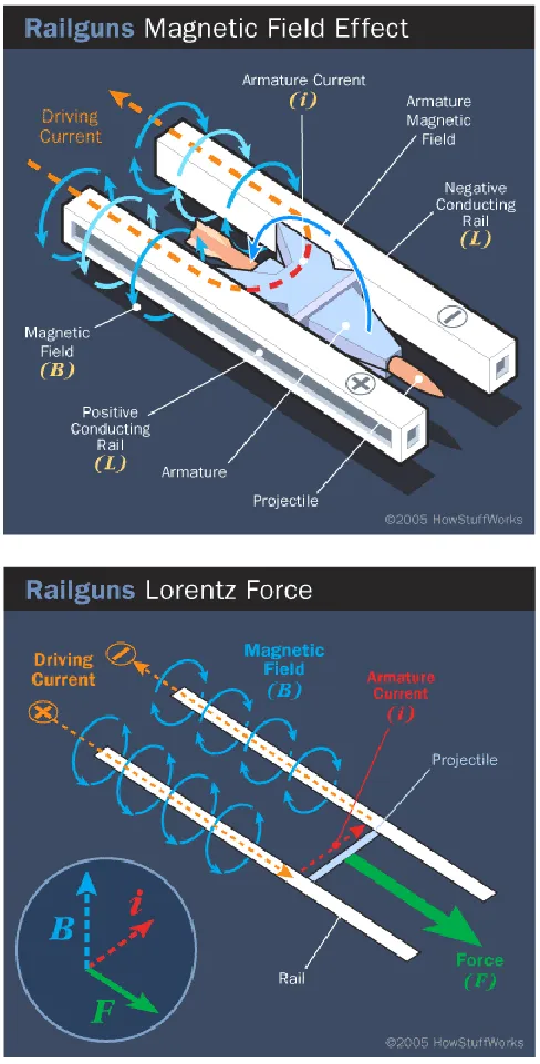
3.3 Electromagnetic Launchers ...59
3.4 Pull-Apart of Gold RF MEMS Asperity Contacts ...61
3.5 Sliding of Asperity Contacts in Electromagnetic Launchers (EMLs) ...71
3.6 References ...75
3.7 Tables and Figures ...80
CHAPTER 4 – MODELING AN F-CENTER WITH THE CHARGE EQUILIBRATION SCHEME ...101
4.1 F-centers ...101
4.2 Charge Equilibration (QEq) Scheme ...105
4.3 Convergence of Lattice Sums ...108
4.4 Charge Distribution with an Anionic Vacancy ...111
4.5 Charge Distribution with an F-center ...112
4.6 Conclusions ...114
4.7 References ...117
LIST OF TABLES
LIST OF FIGURES
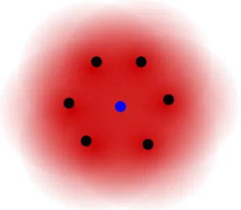
Figure 1.1 Schematic illustration of host atoms’ (black dots) electron density (red cloud) contributing to the binding energy of an “embedded” atom (blue dot). ...21 Figure 1.2 Schematic illustration of the broadening of density of states as the orbitals of two
atoms transition from far apart (a) to overlapped (d). ...22 Figure 1.3 Illustration depicting the different bonding chraacteristics of atoms (red) with the
same coordination (three) but different bond character in two different molecules: (a) graphite; (b) (CH3)2C=C(CH3)2 ...23
Figure 2.1 Figure from Kelchner et al depicting subsurface dislocation loop formation during nanoindentation ...50 Figure 2.2 Multi-scale scheme of Wagner in which the molecular dynamics simulation is
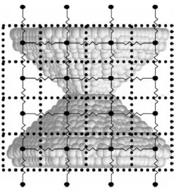
embedded within a finite element domain, and continuum heat flow solutions are conveyed to the atoms at the nodal points. ...51 Figure 2.3 Illustration of the FD/MD multiscale approach in which a network of resistors is
superimposed over an atomistic system, allowing finite difference solutions of
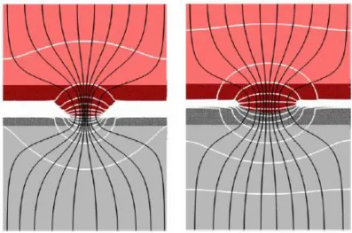
continuum thermal and electrical current to be determined...52 Figure 2.4 Illustration of the increase in current density and heat flow (black lines) and
thermal gradients (white lines) as contact area broadens from left to right. ...53 Figure 3.1 Schematic illustration of basic classes of RF MEMS switches. Left:
Series-configured resistive; Right: Parallel-Series-configured capacitive. ...81 Figure 3.2 Left: SEM image of nanowires on failed gold contact surface; Right: schematic
illustration of a theoretical mechanism for nanowire formation. ...82 Figure 3.3 Schematic illustration of railgun components (top) and operation (bottom). ...83 Figure 3.4 Top: Wear on contact surface of armature: Bottom: molten Al accumulated in
throat of armature. ...84 Figure 3.5 Scale progression of a gold RF MEMS contact surface from (a) fractal model
μm-level topography to (b) nm-μm-level single asperity to (c) atomistic tip with Å-μm-level detail. ...85 Figure 3.6 Illustration of atomistic system for the gold RF MEMS asperity contact
simulations. Atoms colored by local symmetry. Blue indicates bulk, and red
indicates a surface. Crystallographic directions are labeled. ...86 Figure 3.7 Sequential snapshots of a null-voltage simulation of nanowire formation and
fracture during pull-apart of a gold asperity contact. Simulation time is noted in picoseconds. Atoms colored by symmetry; bulk atoms removed...87 Figure 3.8 Snapshot of Thompson tetrahedron forming under the surface after 15
Figure 3.9 Log-log plot of the number of atoms comprising the wire drawn for each initial contact area (blue points) during simulation of pull-apart for gold contacts. A linear regression line fitted to the data is used to extrapolate out to the device-scale contact area of 1x10⁶ nm2 (one square micrometer). ...89 Figure 3.10 Sequential configurations from two gold asperity contact pull-apart simulations.
Top row: 0.1 V; bottom row: 0.2 V. Atoms colored by local symmetry; bulk atoms (blue) present, but transparent. The apparent disorder in the 0.2 V simulation is from thermal noise. ...90 Figure 3.11 Comparison of wire-drawing and deformation after 15 ps of strain for the three
gold asperity contact simulations with Joule heating contribution. Atoms colored by local symmetry. ...91 Figure 3.12 Electrical potential drop across contact as a function of time during gold contact
pull-apart simulation with constant current of 0.01 A and 0.43 V cutoff. ...92 Figure 3.13 Temperature evolution during simulation of gold asperity contact pull-apart.
Top: 0.01 A; bottom: 0.2 V. Atoms colored by temperature as indicated in the scale. ...93 Figure 3.14 Snapshot from simulation of gold asperity contact pull-apart with constant
current of 0.01 A after 16 picoseconds with two-volt cutoff employed. Atoms
colored by temperature as indicated in scale; all atoms in red are above gold’s boiling point of 3239 K. ...94 Figure 3.15 Details for atomistic asperity contact used in aluminum/copper sliding
simulations. ...95 Figure 3.16 Illustration of continuum and atomistic domains for aluminum/copper asperity
sliding simulations. ...96 Figure 3.17 Snapshots of Al (light gray) asperity sliding on Cu (orange) substrate with 0 V
(left) and 0.2 V (right) taken at 5, 10, and 15 picoseconds (top to bottom,
respectively). Atoms with bulk symmetry removed. ...97 Figure 3.18 Close-up view of stacking faults emanating from the base of an Al asperity inside the Al substrate as the asperity slides on Cu. Atoms with bulk symmetry removed. .98 Figure 3.19 Snapshots of Cu (orange) asperity sliding on Al (silver) substrate with 0 V (left)
and 0.2 V (right) taken at 5, 10, and 15 picoseconds (top to bottom, respectively). Atoms with bulk symmetry removed. ...99 Figure 3.20 Close-up snapshot of Cu (orange) atoms dissolving in Al (light gray) during
sliding of a Cu asperity on an Al substrate with 0.2 V applied. Atoms with bulk symmetry removed. Al atoms made transparent. ...100 Figure 4.1 Illustration of Na14Cl131- seed structure. Sodium atoms in red; chlorine atoms in
blue ...122 Figure 4.2 Calculated bulk Madelung constant for center sodium atom as a function of the
Figure 4.3 Illustration of Na4Cl40 seed structure. Sodium atoms in red; chlorine atoms in blue ...124 Figure 4.4 Calculated bulk Madelung constant for center sodium atom as a function of the
number of atoms in a NaCl lattice seeded by the Na4Cl4 cube. Experimental value of 1.74756 is denoted in black ...125 Figure 4.5 Average charge, in electrons, by radial distance from center site of NaCl cube for
(a) sodium atoms and (b) chlorine atoms. Charges labeled in blue refer to the ideal bulk crystal; the red points denote system with anionic vacancy. ...126 Figure 4.6 Average Madelung energy of chlorine atoms by radial distance from the anionic
vacancy in NaCl. ...127 Figure 4.7 Average charges, in electrons, for chlorine atoms by radial distance from the
f-center in NaCl as a function of fixed charge localized in the anionic vacancy. ...128 Figure 4.8 Average Madelung energy of chlorine atoms by radial distance from the f-center
in NaCl. ...129 Figure 4.9 Top: Sum of Madelung energies and self-energies for all ions within 1.5 nm of the
CHAPTER 1 – MOTIVATION
1.1 Classes of atomistic simulations
Atomistic simulations can be conveniently divided into two general classes: 1) quantum mechanical methods that account for electronic structure and 2) classical dynamics methods that replace the electronic structure with appropriate empirical potentials. Each class has its strengths and weaknesses, making the choice of simulation method entirely dependent upon the problem being studied. While the goal of all simulations is to achieve physical accuracy, no model is perfect, and performing theoretical calculations is therefore a task of managing compromises.
Quantum mechanical approaches often include first principles techniques which, as the name suggests, involve the most basic principles of quantum mechanics without
introducing empirical parameters. These approaches attempt to solve the electronic energy levels of atoms to predict physical properties not easily observed, such as binding energies. But solving these energy levels is difficult; an exact solution for Schrödinger’s equation only exists for hydrogen. As the problem expands to multiple atoms multiple interacting nuclei and electrons, approximations must be made to allow for more tractable calculations. The Born-Oppenheimer (BO) approximation1,2 uses the huge nucleus/electron mass ratio to treat the nuclei as stationary relative to the electrons. This allows the electronic wavefunctions to be solved without considering the nuclear degrees of freedom.
many-body wavefunction using N single electron orbitals. The orbital wavefunctions form a Slater determinant4, or matrix of the wavefunctions whose products must satisfy certain physical conditions, namely anti-symmetry with respect to the interchange of electron positions.
While the Hartree-Fock method approaches the quantum mechanical problem through the lens of molecular orbits, an alternative approach is to model energy levels and bonding characteristics using electron density. The Hohenberg-Kohn5,6 theorems state that the physical properties of a many-body system are a functional of the ground-state electron density. This is the basis for density functional theory (DFT) 5,6. DFT calculations are one of the more widely used first principles techniques, and can be carried out by downloadable packages, such as the Vienna Ab Initio Simulation Package (VASP) 7 and
QuantumEspresso8.
Although often powerfully accurate, first principles calculations are extremely computationally demanding with processing power typically scaling with the cube of the system size. In other words, an eight-fold increase in processing resources only nets a two-fold increase in the number of atoms that can be simulated. Because of this, first principles methods are generally restricted to systems containing 102-103 atoms. The size and time scales of many materials science phenomena cannot be captured on such a restricted scale. These processes, including dislocation dynamics and plastic deformation, are better served by simulations using models with more simplistic approximations of electronic structures.
and accelerations and trajectories can then be determined by solving classical equations of motion. Empirical potentials allow for much larger simulation scales in terms of size and time, because the electronic degrees of freedom have been discarded.
Because explicit calculation of electronic states is omitted, construction of suitable empirical potentials is a balancing act between accuracy and transferability. The former entails reproducing physical properties that are consistent with experimental measurements. To accomplish this, empirical potentials are typically fitted to experimental parameters. However, a good empirical potential function must also exhibit transferability, or the ability to reproduce properties to which it was not fitted. Furthermore, these qualities must be achieved while preserving the computational efficiency that makes such potentials attractive. The pursuit of these objectives has led to great advances in the state of the art in empirical potentials; the challenges faced and the solutions that have been developed are detailed in the next section.
1.2 Evolution of empirical potentials
This results in difficulty in modeling the diminishing energetic benefits of forming additional bonds because the weakening of bond strength due to over-crowding, a consequence of Pauli’s principle, is not captured.
The first step towards a many-body representation of atomic bonding energy came in the form of effective medium approximation10. Starting from the result that the energy of hydrogen impurities was primarily dependent on the local environment, Norskov developed an expression for the energy of embedding a defect that treated the “host” material as a gas with density equivalent to the host material, illustrated schematically in Figure 1.1. This gave rise to new understanding of interatomic bonding that would later be utilized in many-body potential energy expressions such as the Finnis-Sinclair (F-S) 11, Embedded Atom Method (EAM) 12, and glue potentials13.
Although derived from different approaches, the F-S, EAM, and glue potentials have the appeal of containing elements of DFT. Recall the Hohenberg and Kohn statement that energy is a functional of electron density. This contribution to potential energy is apparent in the functional form shared by the F-S, EAM and glue potentials. Each is constructed
of atoms to be modeled using only the Cartesian coordinates of its neighbors and thus being much less computationally expensive than explicitly solving electronic energy states.
The functional form of these potentials and that of the Tersoff potential15-17 are essentially the same18. Tersoff developed interatomic potentials for Si and other covalent materials using the energy expression of Abel19, which gives the binding energy as sum of near-neighbor pair interactions modified by the local atomic environment. The local environment term is a function of the local coordination; since nearest-neighbor density changes with the order of a covalent bond, this approximation is successful in describing single-, double- and triple-bond energies in hydrocarbons. However, this environment term encounters difficulties with intermediate bonding systems. Two examples are illustrated in Figure 1.3: graphite and (CH3)2C=C(CH3)2. The atoms in red have the same local coordination
in each molecule, but the bond between them has much different characteristics in one molecule compared to the other. The bond in graphite, due to the conjugated double bonds, has 1/3 double-bond and 2/3 single-bond character; in contrast, the bond in (CH3)2C=C(CH3)2
is purely double-bond in character.
Pettifor subsequently developed an analytic bond order potential21 that circumvented the ad hoc correction terms used by the REBO. Although these corrections eliminated the spurious “averaging” of bond strengths, they added many parameters to the fitting process. Transferability of classical potentials generally suffers as the number of fitting parameters increases. Pettifor’s solution was to explicitly treat π-bonding by going beyond nearest neighbors and including higher moments of electronic bond energy. The second moment describes only the width of an energy distribution (or density of states); the third and fourth moments describe the skewness of the distribution and the tendency to form a gap in the middle of the distribution, respectively. From the standpoint of bond energy, this involves including the contributions of atoms beyond the first shell of nearest neighbors. The moments theorem states that the nth moment of the local density of states is determined by the sum of all paths around neighboring atoms that begin and end at the same atom. The fourth moment approximation includes all neighbors of an atom that can be hopped to and back in four atom-hops or less.
valance bands that span a very narrow range of energies; the energy reduction from
occupying a lower orbital does not offset the exchange energy penalty of changing spin. The result is electrons with aligned spin, giving these metals ferromagnetic properties.
The magnetic contribution to binding energy results in iron taking the bcc phase as its ground state, in contrast to the transition metals ruthenium and osmium, which assume an hcp structure. Therefore, constructing an interatomic potential that captures the quantum mechanical forces behind magnetism is essential for successfully modeling ferromagnetic elements. Pettifor’s higher-moment approximation bond order potential effectively predicts the structural preferences of iron as well as the trend in crystal structures (hcp bcc hcp fcc) that is observed across the non-magnetic 4d and 5d transition metal series.
treatment of electrons. These approaches and their applications are discussed in the next section.
1.3 Multiscale approaches to atomistic simulations
Atomic simulations sufficiently large to model plastic deformation typically require replacing energies from explicit electronic states with some effective inter-atomic potential. The
embedded-atom method (EAM) potentials, for example, have proven to reproduce many of the structural, energetic and vibrational frequencies of a wide range of metals, from which reasonable thermodynamic properties (such as melting temperature) can follow12. At room temperature, however, the thermal transport properties of metals are dominated by electrons, and therefore thermal transport coefficients are not typically reproduced by analytic
potentials. In addition, in a typical large-scale atomic simulation, vibrational modes and phonon states are populated classically, and therefore quantum heat capacities and phonon propagation are not properly treated, again regardless of the quality of the potential energy function.
gold. The resulting temperature profile implies excessively localized heating; the net result will be a tendency to overstate thermally-induced deformation effects.
Several groups have sought to incorporate electronic heat transfer into molecular dynamics simulations using a two temperature model (TTM) 26-32. The TTM decouples electronic and lattice temperatures, and expresses the time evolution of temperatures using nonlinear different equations of continuum heat flow. Solutions to the heat flow equations are typically obtained by finite difference method. When combined with the MD simulation, the lattice temperatures of the TTM are replaced by those calculated from the MD potential, and the electronic temperatures are coupled to the lattice using an electron-phonon scattering mechanism. In an extensive set of studies26-28, Zhigilei and co-workers, for example, have used this concept to model laser interactions with metals. In laser super-heating of metals, where electron temperatures can instantaneously exceed several thousand K, electrons below the Fermi level can be excited and increase the electron-phonon coupling. This makes it difficult to specify a functional form of heat capacity, and heat capacity thus requires density of states calculations.
Rather than using the fine grain two-temperature model to improve thermal transport, one alternative is treat the heat flow dynamics at a scale separate from the atomistic
dynamics. This is conceptually analogous to the multiscale nature of the quasicontinuum (QC) method33. The QC method was developed in order to simulate mechanical properties at longer length scales than what was afforded by atomistic-only simulations, but still
particularly high (e.g. near a point defect); as the mesh size decreases to atomistic
dimensions, force calculations are handed off to an interatomic potential. This methodology was later used to model nanoindentation into a solid with a subsurface grain boundary34.
A potential issue with the QC method is that, while there are multiple size scales simulated, both scales are limited to the time step size of the atomistic simulation. Therefore, stringent limits will be imposed on the material processes that can be simulated. For
example, simulating strain in a crystal will require extremely high strain rates that may not be physically relevant. A multiscale method was developed35 to directly address this limitation by separating the atomistic and continuum simulations. A continuum simulation is run across the entirety of the material volume, while an atomistic simulation is carried out only in a localized region of interest, such as a dislocation. The atomistic forces are then projected to the continuum simulation, allowing for a bridging of the two size scales. And because the two simulations are independent, separate time steps can be used as appropriate for each scale.
The concept of incorporating electronic temperatures combined with a two-scale concurrent simulation approach treating both the atomistic and continuum scales forms the foundation of the methodology developed by Schall et al25. This scheme uses a parallel continuum calculation of heat flow carried out on a grid that is a coarse grained
atom simulation, the thermal transport in the latter is effectively corrected. This methodology was first implemented in simulations of a spherical metallic tip sliding on a silver surface. Without the thermal transport correction from the continuum simulation, the sliding
resistance for the tip was exaggerated due to non-physical localized heating that resulted in melting of the tip.
Describing electronic effects on a continuum scale using experimental input
parameters opens up doors for other capabilities to be introduced into atomistic simulations. Building on this coarse graining approach, Padgett and Brenner36 developed a method in which grid regions are connected by electrical resistors with resistances that are determined from the density and temperature profiles of the atomic simulation. Heat generated from current flow through these resistors is then coupled into the simulation via velocity scaling combined with a local thermostat. Together with the thermal transport corrections, this method is able to introduce Joule heating into a simulation. In addition, because a current flow through the system is known, other effects such as magnetic forces due to current constriction can in principle be included in a simulation.
Another phenomenon that plays an important role in the properties of some materials but which is neglected in most empirical potentials is the role of Coulombic forces arising from atomic charges. Most engineering metals form oxides quite readily, and the
electronegativity differences. Modeling the charge distribution therefore plays a critical role in the simulating metal/metal-oxide interfaces and intermetallic compounds.
An obvious starting point would be to assign fixed charges to atoms at the beginning of a simulation and incorporate the electrostatic energy into the potential function as a constant. However, atomic charges cannot be considered constant for an evolving system. On-site charges in a metallic system containing a surface oxide, for example, will range from near-zero in the bulk metal to nearly fully ionic in the oxide. Hence, accurately describing the Coulombic energy contributions requires the charge states to be continuously solved.
Rappe and Goddard37 developed a method of predicting atomic charges using a method of Charge Equilibration (QEq). The QEq scheme starts from the basis of atoms minimizing chemical potential energy with respect to the addition of charge. The chemical potential for each atom is the derivative of energy with respect to charge, and is a function of empirical parameters derived from atomic data, and an appropriate Coulomb interaction term. This scheme was successfully used to calculate charges on atoms in a variety of organic, inorganic, biological, and polymer systems.
Several groups have incorporated QEq into empirical potentials. Streitz and Mintmire38 combined the QEq methodology with the EAM to simulate aluminum systems containing oxides. The resulting potential accurately described the cohesive, structural, and elastic properties of both fcc aluminum and α-alumina, and the properties of alumina
incorporated into the latter. The charge optimized many-body (COMB) potential39 was developed to simulate Si/SiO2 systems, and was found to effectively predict structures and parameters for silicon and five polymorphs of silica.
The QEq scheme is an approximation of the redistribution of charge, and is not appropriate for all systems. The model allows transferal of partial charges across long distances. For example, when the chemical bond of a HF molecule is broken, the atoms become neutral as the ionization potential of hydrogen exceeds the electronegativity of fluorine. This non-local charge transfer also results in inaccurate polarizability of alkane chains40. This has led to the formulation of charge transfer mechanisms based on pairs of atoms rather than individual atoms. An example is the atom-atom charge transfer (AACT) 40 model that circumvents non-physical long-range charge transfer by constraining transfer of charge to atoms which are directly bonded. The AACT scheme effective fixes some of the problems associated with the entire atomic system being treated as a single conductor. However, the AACT utilizes parameters that are fitted using small structures that are
assumed to be representative of larger and more complex molecules. But this discards one of the more attractive features of the QEq formalism, and that is the use of parameters that are motivated by first principles calculations that likely enhance its transferability.
1.4 Context of current work
processes where the ability to model Joule heating captures physics that would otherwise be inaccessible to an MD simulation. The current work applies the methodology to simulate asperity tips between contacts of various metals in the presence of electromagnetic stress. The multi-scale approach is especially suitable for “hot” metallic contacts, because some of the experimentally-observed deformation effects, such as adhesion and material transfer, are exacerbated with Joule heating. Building back in the thermal physics will allow the
simulations to capture the atomistic detail that eludes typical continuum simulations while still preserving the continuum descriptions of heat flow and electrical current. These “tribological” wear simulations comprise Chapter 3 of the present work.
1.5 References
1. Born M. Quantum mechanics in impact processes. Z Phys. 1926;38(11/12):803-840. doi: 10.1007/BF01397184.
2. Oppenheimer J. On the quantum theory of electronic impacts. Phys Rev. 1928;32(3):0361-0376. doi: 10.1103/PhysRev.32.361.
3. Fock V. Approximation method for the solution of the quantum mechanical multibody problems. Z Phys. 1930;61(1-2):126-148. doi: 10.1007/BF01340294.
4. SLATER J. A simplification of the hartree-fock method. Physical Review. 1951;81(3):385-390. doi: 10.1103/PhysRev.81.385.
5. HOHENBERG P, KOHN W. Inhomogeneous electron gas. Phys Rev B. 1964;136(3B):B864-&. doi: 10.1103/PhysRev.136.B864.
6. KOHN W, SHAM L. Self-consistent equations including exchange and correlation effects. Physical Review. 1965;140(4A):1133-&.
7. Vienna ab initio simulation package (VASP). http://www.vasp.at/2012.
8. Quantum espresso. http://www.quantum-espresso.org/2012.
10.1016/0001-10. NORSKOV J, LANG N. Effective-medium theory of chemical-binding - application to chemisorption. Phys Rev B. 1980;21(6):2131-2136. doi: 10.1103/PhysRevB.21.2131.
11. FINNIS M, SINCLAIR J. A simple empirical N-body potential for transition-metals. Philos Mag A-Phys Condens Matter Struct Defect Mech Prop. 1984;50(1):45-55.
12. Daw MS, Baskes MI. Embedded-atom method - derivation and application to impurities, surfaces, and other defects in metals. Physical Review B. 1984;29(12):6443-6453.
13. ERCOLESSI F, TOSATTI E, PARRINELLO M. Au (100) surface reconstruction. Phys Rev Lett. 1986;57(6):719-722. doi: 10.1103/PhysRevLett.57.719.
14. Sutton AP, Ballufi RW. Interfaces in crystalline materials. Oxford: Clarendon Press; 1995:150-239.
15. TERSOFF J. New empirical-approach for the structure and energy of covalent systems. Phys Rev B. 1988;37(12):6991-7000. doi: 10.1103/PhysRevB.37.6991.
16. TERSOFF J. Empirical interatomic potential for carbon, with applications to amorphous-carbon. Phys Rev Lett. 1988;61(25):2879-2882. doi: 10.1103/PhysRevLett.61.2879.
17. TERSOFF J. Modeling solid-state chemistry - interatomic potentials for multicomponent systems. Phys Rev B. 1989;39(8):5566-5568. doi: 10.1103/PhysRevB.39.5566.
19. ABELL G. Empirical chemical pseudopotential theory of molecular and metallic bonding. Phys Rev B. 1985;31(10):6184-6196. doi: 10.1103/PhysRevB.31.6184.
20. BRENNER D. Empirical potential for hydrocarbons for use in simulating the chemical vapor-deposition of diamond films. Phys Rev B. 1990;42(15):9458-9471. doi:
10.1103/PhysRevB.42.9458.
21. Pettifor D, Oleinik I. Analytic bond-order potentials beyond tersoff-brenner. I. theory. Phys Rev B. 1999;59(13):8487-8499. doi: 10.1103/PhysRevB.59.8487.
22. Drautz R, Pettifor DG. Valence-dependent analytic bond-order potential for transition metals. Phys Rev B. 2006;74(17):174117. doi: 10.1103/PhysRevB.74.174117.
23. Stoner E. Collective electron ferromagnetism. Proc R Soc Lond A-Math Phys Sci. 1938;165(A922):0372-0414. doi: 10.1098/rspa.1938.0066.
24. Los JH, Bichara C, Pellenq RJM. Tight binding within the fourth moment approximation: Efficient implementation and application to liquid ni droplet diffusion on graphene. Phys Rev B. 2011;84(8):085455. doi: 10.1103/PhysRevB.84.085455.
26. Ivanov D, Zhigilei L. Combined atomistic-continuum modeling of short-pulse laser melting and disintegration of metal films. Phys Rev B. 2003;68(6):064114. doi:
10.1103/PhysRevB.68.064114.
27. Lin Z, Zhigilei LV, Celli V. Electron-phonon coupling and electron heat capacity of metals under conditions of strong electron-phonon nonequilibrium. Physical Review B. 2008;77(7):-.
28. Zhigilei LV, Lin ZB, Ivanov DS. Atomistic modeling of short pulse laser ablation of metals: Connections between melting, spallation, and phase explosion. Journal of Physical Chemistry C. 2009;113(27):11892-11906.
29. Gao F, Bacon DJ, Flewitt PEJ, Lewis TA. The effects of electron-phonon coupling on defect production by displacement cascades in alpha-iron. Model Simul Mater Sci Eng. 1998;6(5):543-556.
30. Phillips CL, Crozier PS. An energy-conserving two-temperature model of radiation damage in single-component and binary lennard-jones crystals. J Chem Phys.
2009;131(7):11.
32. Anisimov SI, Kapeliov.Bl, Perelman TL. Electron-emission from surface of metals induced by ultrashort laser pulses. Zhurnal Eksperimentalnoi I Teoreticheskoi Fiziki. 1974;66(2):776-781.
33. Tadmor EB, Ortiz M, Phillips R. Quasicontinuum analysis of defects in solids.
Philosophical Magazine a-Physics of Condensed Matter Structure Defects and Mechanical
Properties. 1996;73(6):1529-1563.
34. Shenoy VB, Miller R, Tadmor EB, Rodney D, Phillips R, Ortiz M. An adaptive finite element approach to atomic-scale mechanics - the quasicontinuum method. J Mech Phys Solids. 1999;47(3):611-642.
35. Wagner GJ, Liu WK. Coupling of atomistic and continuum simulations using a bridging scale decomposition. Journal of Computational Physics. 2003;190(1):249-274.
36. Padgett CW, Brenner DW. A continuum-atomistic method for incorporating joule heating into classical molecular dynamics simulations. Molecular Simulation. 2005;31(11):749-757.
37. Rappe AK, Goddard WA. Charge equilibration for molecular-dynamics simulations. J Phys Chem. 1991;95(8):3358-3363.
39. Yu J, Sinnott SB, Phillpot SR. Charge optimized many-body potential for the si/SiO2 system. Phys Rev B. 2007;75(8):085311. doi: 10.1103/PhysRevB.75.085311.
1.6 Tables and Figures
Figure 1.2 Schematic illustration of the broadening of density of states as the orbitals of two atoms transition from far apart (a) to overlapped (d).
# of States
Orbit
al
Ener
gy
(a)
(b)
(a) (b)
Figure 1.3 Illustration depicting the different bonding characteristics of atoms (red) with the same coordination (three) but different bond character in two different molecules: (a)
CHAPTER 2 – THEORY AND MODELING METHODS
In this chapter, the underlying principles of the methodologies utilized in Chapters 3 and 4 are reviewed in detail. The purpose of this chapter is to proceed through the background of each modeling technique to provide a theoretical justification for their present
implementation. The computational details, parameters, and obstacles of typical simulations are outlined for each application.
2.1 Embedded Atom Method
Early classical dynamics simulations often used two-body pair potentials which express the energy for a collection of bodies as pair-wise additive. Different functional forms of this interaction have been specified. For example, the Lennard-Jones1 potential gives the two-body energy as
( ) [( ) ( ) ] (2.1)
where r is the distance between the atoms, ε is the equilibrium energy minimum for the pair, and σ is the distance at which V(r) is equal to zero. The first term in the bracket describes the energy contribution from Pauli repulsion which occurs at short ranges due to overlapping electron orbitals; the second term in the brackets represents the long-range, cross-atomic attractive contribution. The Morse potential2 similarly expresses pair interaction using competing repulsive and attractive components,
where ρ and ε are equilibrium bond length and dislocation energy, respectively, and β is an inverse length scaling factor that endows the Morse potential with more intermediate range of interaction. The exponential-6 potential3 modifies the Lennard-Jones potential by substituting a repulsive term with exponential form
( ) (2.3)
where A, B, and C are constants. The exponential term more appropriately captures the decay of intermolecular repulsions.
Pair potentials of these forms have severe limitations in predicting properties of crystalline solids stemming from the inability to capture the influence of local atomic environment on bonding. Intuitively, the energetic favorability of atomic bonding should diminish with increasing atomic density, and this is ignored in typical pair potentials. Pair potentials also do not account for directionality in bonding, as the interaction terms are dependent only on the distance between two atoms. Consequently, covalent bonding is not properly captured by pair potentials. These two limitations can result in highly inaccurate cohesive energies and elastic constants in metals.
One solution proposed4 to capture atomic environment contributions was to augment a pair potential expression with a volume term, such that
( ⁄ ) ∑ ( ) (2.4)
definitive quantity for the volume to be known. This poses potential problems for systems with ambiguities in the total volume, as is the case for surface relaxations, point defects, and fracture surfaces.
The EAM5 is an expression for energy that combines a pair interaction term with an embedding term that more explicitly treats the local environment dependence of atomic energy. This approach essentially treats all atoms as impurities, and a contribution to energy is obtained from each impurity disturbing the electron density of the local environment. The functional form for the energy of atom i due to j neighbors is
∑ ( ) ∑ ( ) (2.5)
where F is the embedding energy of atom i, is the electron density at site i, and is the pair interaction for neighbor j at a distance . This has the appealing characteristic of being philosophically rooted in density functional theory (DFT) principles, since the energy is being described as a functional of the atomic-like electron density6.
The embedding energy function and pair potential are determined empirically from physical properties of the solid. Foiles et al7 derive these for several fcc metals, including Au, Cu and Ni, using the lattice constant, elastic constants, vacancy-formation energy, and sublimation energy in fcc and bcc phases. The embedding energy can be uniquely specified by fitting the energy from Eq. 2.5 to Rose’s equation of state8
( ) ( ) (2.6)
( ) (
)
(2.7)
where B is the bulk modulus, is the equilibrium volume per atom, and a and a0 are the fcc
lattice constant and equilibrium lattice constant, respectively. Then, all one needs to specify for the embedding function is the electron density, which is obtained from atomic densities computed from the Hartree-Fock wave functions by
( ) ( ) ( ) (2.8)
where and are the number of s and d electrons (the bonding electrons for transition metals), respectively, and and are the densities associated with the s and d wave functions. The sum is fixed for a given metal, and is varied for the fitting procedure. The pair potential is expressed as
( ) ( ) (2.9)
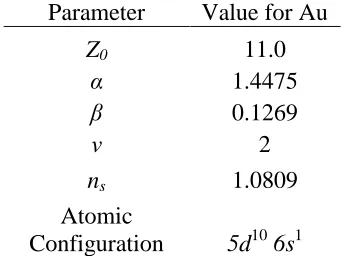
where is the number of outer electrons, and , , and are fitting parameters. The parameters are determined primarily by the shear moduli and vacancy-formation energy; the ones used for the Au EAM potential are given in Table 2.1.
Since its introduction, the EAM has been an important tool in atomistic simulations of nanoscale metallic properties. For example, Landman et al used the EAM to simulate the deformation of asperity tips to obtain a better understanding of how macroscopic scale contact mechanics apply to interfaces when the size scale is sufficiently small12. The
indentation and pull-off of Au and Ni pyramidal asperity tips was modeled using tips with an effective radius of about 30 angstroms. A “jump to contact” phenomenon during indentation was noted in which adhesion occurs by displacement of tip atoms, with a deformation
method and pressure distribution similar to those predicted by contact mechanics theories. Pull-off of the asperity tips resulted in a “neck” that maintained crystalline structure, and the normal force through the neck was relatively constant during deformation, which is
consistent with what would be predicted at the continuum level.
Kelchner et al. 13 explored the capability of the EAM to resolve atomistic details of nanoindentation processes by treating the asperity tip as a purely repulsive element. This prevents the adhesive forces between tip and substrate that produce a “jump to contact” phenomenon, an effect that is not necessarily realistic because real indenters have unclean surfaces and hence much lower adhesion energies than clean metallic surfaces. The simulations by Kelchner showed that the nanoindentation force initially follows the
2.2 Molecular Dynamics Simulations
Atomistic simulations with interatomic potentials use integration of classical equations of motion to determine the accelerations, velocities, and positions of atoms from the potential energy. At each time step in the simulation, the forces on the atoms are evaluated, and the system is evolved one timestep using a numerical integration scheme; for the current work, the numerical integration is completed using a Gear predictor-corrector algorithm. This algorithm uses up to fourth order time-derivatives of the current atomic positions to predict the positions of atoms at the next time step. The atoms temporarily “step” to these predicted positions, and forces computed from the potential at these positions are compared to the forces from the prediction stage. The differences between the new forces and the predicted forces are then used to correct the trajectory, and the positions are the next time step are then determined.
An alternative to the predictor-corrector algorithm is to integrate the equations of motion using the velocity Verlet algorithm. The velocity Verlet uses velocities and
The time step used for the integrator is one femtosecond. The selection of time step size for the integrator is system dependent, as it is required to be at least ten times shorter than the duration of the fastest motion in the system. Vibrations in molecules can have periods as short as ~10-14 s. This sets the upper bound for the time step size in a typical molecular dynamics (MD) simulation to ~10-15 s. The MD simulations reported here are typically run for a duration of ~100 picoseconds, or 100,000 time steps.
Basic MD simulations run in NVE, where the number, volume, and total energy are constant throughout the simulation. Consequently, the atoms experience fluctuations in temperature defined by average kinetic energy. However, it is often desirable to maintain a specified temperature in the system based on prescribed conditions or, as we will see later, feedback from external degrees of freedom. The simplest method of fixing atomistic temperatures is by re-scaling the velocities15 to “correct” the current temperature to the desired temperature. Although appealing from the standpoint of coding difficulty, velocity scaling potentially introduces non-physical effects, including localized, correlated motion. In addition, since the temperature is fixed over time, it does not produce fluctuations in
temperature as required by statistical mechanics.
minimization of differences between free and constrained accelerations. The term is incorporated into the equations of motion as follows:
, (2.10)
∑ ∑ ⁄ (2.11)
where F, v, and m, are the force, velocity, and mass, respectively. The frictional term, , can be negative or positive for atoms depending on what is required to maintain constant temperature. The summation is typically over all atoms, but as will be shown later, the thermostat can be used in local regions of an MD simulation.
2.3 Continuum Principles of Current Flow at Metal-Metal Contacts
The physics for electrical contacts has been studied extensively17. The roughness of contacts creates groups of separate contact spots, known as a-spots. When an electrical current is present, the current flow lines distort to enter a contact spot. This creates a resistance, because the flow line constriction dictates that only a finite amount of electrical current may pass through a given contact spot. This is known as the constriction resistance, and for a circular contact with radius a much larger than the electron scattering length, it can be calculated as
Rc = ρ/2a (2.12)
where ρ is the material resistivity.
current flow lines. An increase in the Joule heating due to a higher current density through an asperity is accompanied by a commensurate increase in heat flow due to a larger thermal gradient. Hence, the temperature increase is a function of the voltage applied, giving rise to the voltage-temperature relationship. Assuming the thermal conductivity and electrical resistivity, λ and ρ, respectively, are linearly dependent on temperature, the expression for temperature increase in a conductor with potential V applied is
(2.13) where β and α are, respectively, the temperature coefficients of thermal conductivity and electrical resistivity. The quantity T1 represents the bulk temperature of the conductor, and Tm
is the maximum superheated temperature at steady state for the given voltage. A simplified version of this V-T relation may be attained by exploiting the Wiedemann-Franz Law. This law expresses the temperature variations of thermal conductivity and electrical resistivity as
(2.14) where L is the Lorentz constant 2.45x10⁻⁸ V2 K-2. This law applies well to many conducting materials, and allows Equation 2.13 to be reduced to
(2.15) This relationship underscores an important corollary of the overlap of heat flow lines and electrical current lines. Reduction in the size of an electrical contact produces a higher current density for a given voltage, but does not increase the equilibrium temperature at the contact because the heat flow lines also become denser and consequently produce steeper
} 3 / ) ( 2 / ) )( ( ) {( 8 3 1 3 2 1 2 1 0 0 2 T T T T T T
V m m m
LT
V2=
thermal gradients. The by-product of this is that the voltage required to melt (or boil) an electrical contact is an intrinsic material property without regard to the contact scale at equilibrium. Gold, for instance, melts at 1,337 K, which equates to an electrical potential drop of 0.43 V.
Although the maximum steady-state temperature in a conductor is fixed given the applied voltage, the time needed to reach this temperature is not, and is highly dependent on the voltage itself. The reduced time (μs/μm2
) for reaching steady state can be expressed as17
[ [
]] (2.16)
where V is the applied voltage, Teq is the equilibrium temperature from Equation 2.13, T0 is
the bulk temperature of the conductor, and α is a constant equal to 41.7852 μm/[V μs]0.5 . The time needed to reach the steady-state temperature is thus inversely proportional to the applied voltage, and proportional to the contact area.
2.4 Continuum-Atomistic Thermostat
There have been many other approaches in the past to build back in electronic effects that are not well described by empirical potentials. Zhigilei and others19-21 have combined the two-temperature model (TTM) with MD simulations in study laser heating of materials. This is a challenging application to model, because there are disparate sets of physics involved. For instance, the laser interaction in metals produces extremely rapid heating that exceeds the pace at which thermal energy can be transferred from electrons to phonons, requiring a description of electronic temperatures. On the other hand, the thermal energy deposition potentially induces microstructural changes, such as phase transformations, that are well-suited to atomistic simulation. The hybrid TTM-MD model by Zhigilei de-couples the lattice and electronic temperatures, allowing the former to be modeled by the MD simulation and the latter by the TTM. An electron-phonon scattering mechanism allows coupling between the electron temperatures and the lattice.
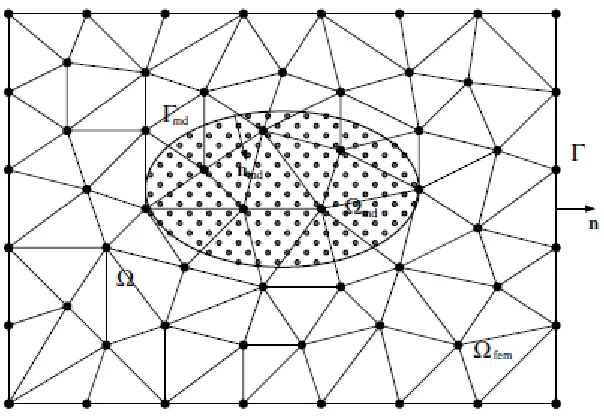
Wagner developed a continuum-atomistic technique22,23 motivated by the desire to extend the thermal boundaries of a system beyond what is computationally feasible for an all-atomistic system. This scheme allows thermal energy to be passed back and forth between a small atomistic system and a surrounding continuum body, as illustrated schematically in Figure 2.2. Heat flow in the continuum region is governed by Fourier’s heat law, and uses experimental density, heat capacity and thermal conductivity, and is conveyed to the atomistic region by augmenting the interatomic potential energy used for the molecular dynamics simulation.
continuum simulation to project continuum heat transfer properties onto a concurrent atomistic simulation. In this ad hoc technique, a network of static, cubic grids is superimposed over the atomistic system. The grids contain continuously updated
temperature, density and composition profiles determined by the atomistic simulation. The temperature of each grid section, for example, is equated to the average kinetic energy
(minus the center of mass velocities) of the atoms in that grid section. Using this temperature distribution, new temperatures for the grid regions are then calculated by numerically solving the continuum heat flow equation of the form
(2.17)
where T is the temperature derived from the MD simulation, and D is the experimental thermal diffusivity.
In the original implementation of this methodology18, Equation 2.17 was evaluated explicitly via Euler’s method, using a forward difference time derivative with a step size on the order of the MD simulation time step (~1 femtosecond). To preserve stability in the time derivative, the time step size is bounded by a maximum governed by the size of the finite difference grids and the value for D as
( ) (2.18)
A more recent version of the methodology uses thermal resistors for heat flow to circumvent the time step limitations induced by numerical instability. The use of thermal resistor-capacitor (RC) circuits is a common way of solving continuum heat transfer27. Resistance, the product of voltage drop and current in electrical terms, can be analogously defined in thermal terms by replacing voltage drop with temperature differential, ΔT, and current flow with heat flow, q. Thermal resistance for the grid boxes is thus defined as
( ) (2.19)
where L is the length of the box whose thermal resistance is defined , is the thermal conductivity, and A is the area of the box. Thermal capacitance of the grid is given by cp x ρ
x V, where cpis the heat capacity of the material, ρ is the density, and V is the grid volume.
Using these definitions, heat flow within the thermal circuit can be solved using Kirchoff’s laws. Once the continuum temperatures in each grid are determined, they are communicated to the atoms by rescaling the atomic velocities. The integration of the atomic equations of motion is stepped forward in time one step while applying a Hoover thermostat locally to each grid region. The grid profiles are then recalculated and this feedback process between the atomic and continuum simulations is repeated as the simulation progresses.
allowing heat to flow into the potential energy modes while maintaining an appropriate thermal profile. While perhaps unsatisfactory from a formal viewpoint, this is a pragmatic approximation for the simulations.
In addition to the thermal resistors connecting the continuum grid boxes, an electrical resistor network is implemented to model electrical potential drop and current flow. This differentiates the current methodology from the previous multi-scale techniques that
primarily dealt with heat flow properties, and builds in the capability to model Joule heating through a continuously evolving atomistic system. As with the thermal properties, the electrical resistance of each grid region is calculated using information from the atomistic simulation. Based on the density profile of the grid, a resistivity is computed using the temperature-dependent experimental bulk resistivity for the material. For regions containing more than one species of atom, averaged bulk properties are used, while for regions that are devoid of atoms, the resistance of air is used. The virtual electrical resistors that connect neighboring grid regions then are assigned a resistance taken as the average resistance of the grid regions that they connect. An illustrative example of resistor grid construction is illustrated in Figure 2.324.
calculated first for a given voltage without coupling to the atoms. The voltage is then
adjusted and the current is recalculated. This procedure is continued until the desired current is attained within some pre-specified error. The coupling with the atomic dynamics is then resumed as detailed above. The experimental thermal and electrical transport values in the continuum simulations are taken from Slade28.
A key advantage to the methodology utilized in this work is the flexibility it affords in system configurations. When the atomic and continuum simulations are carried out concurrently, the same step size is used to solve the atomic equations of motion as is used to numerically solve the current and heat transport equations via the resistor networks.
However, a larger time step size can also be used with the virtual resistor system. This becomes particularly important in the case of Joule heating at a small contact, where the steady state thermal conditions are preceded by a transient period of heat flow. The rate at which the thermal transients give way to steady state conditions is determined by the thermal time constant, which is directly proportional to the heat capacity of the material and the thermal resistance. As Equation 2.19 implies, a narrow dimension (i.e. a small electrical contact) produces a large thermal resistance, which in turn lengthens the period of time before steady state thermal conditions. This necessitates a continuum-only “run-in” period of ~10-100 nanoseconds to determine the steady state thermal conditions. These conditions are then coupled to the atoms for the beginning of the atomistic simulation.
simulation. Flow lines for electrical current and heat contort to enter a constriction point such as an asperity contact. Upon exiting the constriction, the flow lines spread out to ultimately re-attain geometry perpendicular to the contact. Figure 2.4 illustrates this for the simulations of Joule heating through aluminum-copper asperity contacts carried out by Irving25. The darkened portions near the contact comprise the volume treated by the atomistic simulation and amount to approximately 15 nm in the contact direction. The lighter regions represent continuum volumes for the respective materials and have
thicknesses five times greater than the contact substrates. As one can see from the flow lines represented by the black lines, the influence of the constriction on the spread of the flow lines extends well beyond the atomistic region. Therefore, applying the same boundary for both the continuum and atomistic simulations would introduce unphysical effects into the continuum solutions. In the case of a fixed temperature boundary, as utilized by Irving, the effect would be one of an artificially high thermal gradient. Therefore, the finite difference grid for the continuum simulation is typically displaced far from the atomistic region.
2.5 Charge Equilibration
Atomic charges in MD simulations are typically fixed. For systems with interfaces or phases with ionic bonding characteristics, this potentially introduces unrealistic treatment of the bond energies. The charge equilibration (QEq) approach taken by Rappe and Goddard29 computes the optimum charge distribution of a system by minimizing the total energy with respect to on-site charges. The QEq scheme serves as the basis for the treatment of charge in
The on-site energy of an atom with respect to charge can be expanded as a Taylor series as follows32:
( ) ( ) ⁄ ( ) (2.20)
When =-1, the energy is equivalent to the electron affinity; when =+1, the energy is the ionization potential. Using these solutions, the first and second-order derivatives become
( ) ⁄ ( ) (2.21)
( ) (2.22)
The first derivative term is the electronegativity; the second derivative is known as a hardness, or self-Coulomb33, and represents repulsion between two electrons in a valence orbital. The local atomic energy can thus be expressed as29,30
(2.23)
where is the electronegativity of atom i and is the self-Coulomb. The total electrostatic energy can then be described as
(2.24)
with Jij the Coulomb interaction between centers i and j resulting from overlapping charge
distributions.
The optimum charge distribution corresponds to the equilibrium at which the atomic chemical potentials, or change in each atom’s energy with respect to its charge, are
equalized:
0 1 0 2
( )
2
i
i i i i i
E q q J q
1 ( )
2 i
es ij i j
i i j
E E q J q q
(2.25)
where χA is the chemical potential of atom A. Under the constraint that the N atom charges
must sum to the total system charge,
∑ (2.26)
one is left with N simultaneous equations of the form where Q is a vector of all the charges, the components of C are
(2.27)
for I ≥ 2 (2.28) and the components of D are
(2.29)
for I ≥ 2 (2.30)
Rappe and Goddard proposed a method for constraining the charge solutions within a prescribed range. For instance, the charge on a lithium atom is required to be greater than -7, but less than +1. To enforce this constraint, the charge solutions obtained from Equations 2.27 – 2.30 are compared to the permitted range. A charge falling outside the range is set to the boundary limit. The equations are then re-solved for N – p atoms, where p is the number of atoms for which charge has been fixed. The components of D from Equations 2.29 and 2.30 then become
∑ (2.31)
0 0
1
( ... )
A N A AA A AB B
B A
q q J q J q
...
A B C N
where
∑
for I ≥ 2 (2.33) and the charges on the non-fixed atoms are then solved. While charges for the NaCl crystals in the present work do not move outside of reasonable boundaries, this reduced equation methodology later will be shown to be important for modeling the extra electron of an f-center.
The values for and are derived from atomic data29; the two-center Coulomb interaction, Jij, on the other hand, requires an assumption about the atomic charge densities.
Assuming point charge interaction proportional to 1/R (Coulomb’s law) is valid for atoms at large separation but approaches infinity for atoms that are closely spaced. Slater-type29 and Gaussian-type30 orbitals have been implemented in the QEq, which correct for overlapping charge densities. However, computing these orbitals continuously for a large number of atoms is impractical from a computational resource standpoint. A less computationally-demanding alternative is to express the Coulomb interaction using an approximation. Oda and Hirono34 compared several forms for this approximation; the present work utilizes the form for that was found to be the most accurate and transferable, the DasGupta-Huzinaga (DH) equation35
(2.34)
where is the distance between the atoms.
2.6 References
1. Lennard-Jones JE. Proc R Soc Lond A. 1924;106:463.
2. Morse P. Diatomic molecules according to the wave mechanics. II. vibrational levels. Phys Rev. 1929;34(1):57-64. doi: 10.1103/PhysRev.34.57.
3. Buckingham R. The classical equation of state of gaseous helium, neon and argon. Proc R Soc Lond A-Math Phys Sci. 1938;168(A933):264-283. doi: 10.1098/rspa.1938.0173.
4. JOHNSON R. Relationship between 2-body interatomic potentials in a lattice model and elastic-constants. Physical Review B. 1972;6(6):2094-&. doi: 10.1103/PhysRevB.6.2094.
5. Daw MS, Baskes MI. Embedded-atom method - derivation and application to impurities, surfaces, and other defects in metals. Physical Review B. 1984;29(12):6443-6453.
6. HOHENBERG P, KOHN W. Inhomogeneous electron gas. Phys Rev B. 1964;136(3B):B864-&. doi: 10.1103/PhysRev.136.B864.
7. Foiles SM, Baskes MI, Daw MS. Embedded-atom-method functions for the fcc metals cu, ag, au, ni, pd, pt, and their alloys. Physical Review B. 1986;33(12):7983-7991.
9. Liu G, Zhang GJ, Ding XD, Sun J, Chen KH. Modeling the strengthening response to aging process of heat-treatable aluminum alloys containing plate/disc- or rod/needle-shaped precipitates. Mater Sci Eng A-Struct Mater Prop Microstruct Process. 2003;344(1-2):113-124.
10. ERCOLESSI F, ADAMS J. Interatomic potentials from 1st-principles calculations - the force-matching method. Europhys Lett. 1994;26(8):583-588. doi:
10.1209/0295-5075/26/8/005.
11. ROHRER C. Interatomic potentials for al-cu-ag solid-solutions. Modell Simul Mater Sci Eng. 1994;2(1):119-134. doi: 10.1088/0965-0393/2/1/009.
12. LANDMAN U, LUEDTKE W, RINGER E. Atomistic mechanisms of adhesive contact formation and interfacial processes. Wear. 1992;153(1):3-30. doi:
10.1016/0043-1648(92)90258-A.
13. Kelchner CL, Plimpton SJ, Hamilton JC. Dislocation nucleation and defect structure during surface indentation. Physical Review B. 1998;58(17):11085-11088.
14. Allen MP, Tildesley DJ, eds. Computer simulation in chemical physics. Dordrecht ; Boston: Kluwer Academic Publishers; 1993.
http://www2.lib.ncsu.edu/catalog/record/DUKE001118237.
16. Hoover WG. Molecular dynamics lecture notes in physics. Berlin: Springer-Verlag; 1986.
17. Timsit RS. Electrical contact resistance: Properties of stationary interfaces. Ieee Transactions on Components and Packaging Technologies. 1999;22(1):85-98.
18. Schall JD, Padgett CW, Brenner DW. Ad hoc continuum-atomistic thermostat for modeling heat flow in molecular dynamics simulations. Molecular Simulation. 2005;31(4):283-288.
19. Ivanov D, Zhigilei L. Combined atomistic-continuum modeling of short-pulse laser melting and disintegration of metal films. Phys Rev B. 2003;68(6):064114. doi:
10.1103/PhysRevB.68.064114.
20. Zhigilei LV, Lin ZB, Ivanov DS. Atomistic modeling of short pulse laser ablation of metals: Connections between melting, spallation, and phase explosion. Journal of Physical Chemistry C. 2009;113(27):11892-11906.
21. Lin Z, Zhigilei LV, Celli V. Electron-phonon coupling and electron heat capacity of metals under conditions of strong electron-phonon nonequilibrium. Physical Review B. 2008;77(7):-.
23. Wagner GJ, Jones RE, Templeton JA, Parks ML. An atomistic-to-continuum coupling method for heat transfer in solids. Comput Methods Appl Mech Eng. 2008;197(41-42):3351-3365. doi: 10.1016/j.cma.2008.02.004.
24. Padgett CW, Brenner DW. A continuum-atomistic method for incorporating joule heating into classical molecular dynamics simulations. Molecular Simulation. 2005;31(11):749-757.
25. Irving DL, Padgett CW, Brenner DW. Coupled molecular dynamics/continuum simulations of joule heating and melting of isolated copper-aluminum asperity contacts. Modell Simul Mater Sci Eng. 2009;17(1):-.
26. Irving DL, Padgett CW, Guo Y, Mintmire JW, Brenner DW. Multiscale modeling of metal-metal contact dynamics under high electromagnetic stress: Timescales and
mechanisms for joule melting of al-cu asperities. IEEE Trans Magn. 2009;45(1):331-335.
27. Fundamentals of heat and mass transfer. Hoboken, NJ: John Wiley; 2007. http://www2.lib.ncsu.edu/catalog/record/DUKE003789783.
28. Timsit RS. Slade PG, ed. Electrical contacts: Principles and applications. New York: Marcel Dekker; 1999.
30. Streitz FH, Mintmire JW. Electrostatic potentials for metal-oxide surfaces and interfaces. Physical Review B. 1994;50(16):11996-12003.
31. Yu J, Sinnott SB, Phillpot SR. Charge optimized many-body potential for the si/SiO2 system. Phys Rev B. 2007;75(8):085311. doi: 10.1103/PhysRevB.75.085311.
32. Iczkowski R, Margrave JL. Electronegativity. J Am Chem Soc. 1961;83(17):3547-&.
33. Parr RG, Pearson RG. ABSOLUTE HARDNESS - COMPANION PARAMETER TO ABSOLUTE ELECTRONEGATIVITY. J Am Chem Soc. 1983;105(26):7512-7516.
34. Oda A, Hirono S. Geometry-dependent atomic charge calculations using charge equilibration method with empirical two-center coulombic terms. Theochem-J Mol Struct. 2003;634:159-170. doi: 10.1016/S0166-1280(03)00338-5.
2.7 Tables and Figures
Table 2.1 Parameters used for fitting the pair interaction in the Embedded Atom Method potential for Au7.
Parameter Value for Au
Z0 11.0
α 1.4475
β 0.1269
ν 2
ns 1.0809
Atomic
CHAPTER 3 – ASPERITIES UNDER ELECTROMAGNETIC STRESS
3.1 Nanotribology
The surfaces of contacting metals contain nanoscale protrusions, or asperities, through which contact forces are transmitted. In an electrically conducting interface, the asperities become the conduits of current. It is known that plastic deformation of the asperities influences the contact area 1, which in turn alters contact resistance. Therefore, understanding the
mechanisms of asperity wear is critical to ensuring the integrity of electrical contacts
The role of asperities in nanotribology is well-studied 2, particularly in the domain of modeling. Nanoindentation of metals, in particular, has been the subject of many molecular dynamics (MD) simulations. Li et al 3 modeled the indentation of a flat <111> Al surface using a spherical indenter and witnessed glide loops emanating on three equivalent
{111}<110> slip systems. A similar simulation of the indentation of a (111) Au surface by Kelchner and colleagues 4 also produced dislocation loops, but without the same three-fold symmetry witnessed by Li. The presence of surface steps during nanoindentation of (100) Al was found by Hirel et al 5 to strongly influence the critical size for a stable dislocation half-loop, below which a dislocation will retreat back to the surface. Indentation of a (111) Au surface with steps performed by Zimmerman 6 indicated that close proximity to a surface step resulted in a greater dependence on the crystallographic orientation for dislocation
morphology.