Forecasting Malaysia Load
Using a Hybrid Model
NORIZAN MOHAMED
1, MAIZAH HURA AHMAD
21Mathematics Department, Faculty Of Science And Technology, Universiti Malaysia Terengganu (UMT),
21030 Kuala Terengganu, Terengganu, MALAYSIA.
2Department of Mathematics, Faculty Of Science, Universiti Teknologi Malaysia, 81310 UTM Skudai,
Johor, MALAYSIA.
E-mail: [email protected], [email protected]
ABSTRACT
A hybrid model, which combines the seasonal time series ARIMA (SARIMA) and the multilayer feed-forward neural network to forecast time series with seasonality, is shown to outperform both two single models. Besides the selection of transfer functions, the determination of hidden nodes to use for the non linear model is believed to improve the accuracy of the hybrid model. In this paper, we focus on the selection of the appropriate number of hidden nodes on the non linear model to forecast Malaysia load. Results show that by using only one hidden node, the hybrid model of Malaysia load performs better than both single models with mean absolute percentage error (MAPE) of less than 1%. Keywords: Load Forecasting; Seasonal Autoregressive Integrated Moving Average; Multilayer Feed-forward Neural Network; Hybrid Model; Hidden Nodes.
1. INTRODUCTION
An important area of forecasting is time series forecasting where the model of an observed time series is developed to forecast the future values. Load demand is one of the time series data and it is one of the major input factors in economic development especially in a developing country such as Malaysia. Forecasting load demand with accurate forecast is hoped to help our country, especially the Department of Operation and Planning (Tenaga Nasional Berhad, Malaysia) to generate an appropriate load of required power supply.
One of the most important and widely used time series models is the autoregressive integrated moving average (ARIMA) model. An ARIMA process combines three different processes comprising an Autoregressive (AR) functions regressed on the past values of the process, moving average (MA) functions regressed on a purely random process with mean zero and variance σ2 [6] and an integrated (I) part to make the data series stationary by differencing
[6][20]. The ARIMA model is extended in order to handle seasonal aspects of time series, and the general notation is ARIMA(p,d,q)(P,D,Q)swhere (p,d,q)is the non-seasonal part of the model,
) , ,
(PDQ is the seasonal part of the model and s is the seasonal length with abbreviated as seasonal ARIMA, SARIMA [11].
Working with few hidden nodes saves time in training the network. However, if a network is defined with too few hidden nodes, the network probably would not train at all or train with an unreliable forecasting because of the inability of the network to reproduce the system dynamics accurately [7][9]. If we defined just enough hidden nodes, the network may train but it might not be robust in the face of noisy data, or it would not recognize new patterns [7]. Too many hidden neurons, in the best case, will provide reliable forecasting, but with an excessive computing time and a high memory consumption, while, in the worse case, will only learn the presented patterns and will not be able to generalize the acquired knowledge to predict new patterns [7][9]. Therefore, the selection of the appropriate number of hidden nodes is not an easy task to get back-propagation neural network to train successfully.
The main purpose of this study is to show that a hybrid model can overcome the problem of selecting the appropriate number of hidden nodes and hence improve forecasts produced by two single methods, namely SARIMA and multilayer feed-forward neural network. The current paper presents a hybrid model with a selection between 1 to 19 hidden nodes for the non linear model.
The remainder of this paper is organized as follows. In section 2, we present the Box-Jenkins seasonal ARIMA model and the multilayer feed-forward neural network model. The hybrid model is presented in section 3. In section 4, details of the results are discussed. Finally in section 5 we give our conclusions.
2. FORECAST METHODOLOGY
A variety of different forecasting approaches is available to forecast time series data and it is important to realize that no single model is universally applicable [5]. Two approaches presented here are the Box-Jenkins seasonal ARIMA (SARIMA) and the multilayer feed-forward neural network models.
2.1 Box-Jenkins Seasonal ARIMA (SARIMA) Model
In practice, many time series contain a seasonal periodic component, which repeats every s observation. To deal with seasonality, the ARIMA model is generalized hence a general multiplicative seasonal ARIMA (SARIMA) model is defined [2][3] which follows the ARIMA general procedure represented as follows:
t s Q q t D s d s P
p
(
B
)
Φ
(
B
)(
1
−
B
)
(
1
−
B
)
Z
=
θ
(
B
)
Θ
(
B
)
a
φ
&
(1)with Qs Qs s s s s s Q q q q Ps Ps s s s s s P p p p
B
B
B
B
B
B
B
B
B
B
B
B
B
B
B
B
Θ
−
−
Θ
−
Θ
−
=
Θ
−
−
−
−
=
Φ
−
−
Φ
−
Φ
−
=
Φ
−
−
−
−
=
L
L
L
L
2 2 2 2 1 2 2 2 2 11
)
(
,
1
)
(
,
1
)
(
,
1
)
(
θ
θ
θ
θ
φ
φ
φ
φ
where B denotes the backward shift operator and at denotes a purely random process.
The original series Zt is differenced by appropriate differencing to remove non-stationary terms. d
B) 1
( − and (1−Bs)D are the seasonal and non-seasonal differencing operators, respectively [11].
2.2 Multilayer Feedforward Neural Network
The multi-layer feed-forward neural network (MFNN) is a well known neural model, which consists of an input layer, one or several hidden layers and an output layer. The neurons in the feed-forward neural network, are generally grouped into layers. Signals flow from the input layer to the output layer via unidirectional connections, the neurons being connected from one layer to the next, but not within the same layer [15].
An essential factor of successes of the neural networks depends on the training network. Among the several learning algorithms available, back-propagation has been the most popular and most widely implemented learning algorithm of all neural networks paradigms [4][5]. Among the advantages of back-propagation (BP) is its ability to store numbers of patterns that exceed its built-in vector dimensionality [4]. Basically, the BP training algorithm with three-layer feed-forward architecture means that, the network has an input layer, one hidden layer and an output layer. More hidden layer can be used but three layers are sufficient to enable this type of network to model any deterministic process within reasonable limit [18].
Neural network function sends the vector
(
x1,L,xN)
in RN to the vector(
y1,L,yM)
in RM. Thus, the feed-forward network can be represented as [18]:( )
x
F
y
=
(2)where x=(x1,L,xN) and y=
(
y1,L,yM)
. The values yk for the feed-forward network with N input nodes, H hidden layer nodes and M output nodes are given by [8]:M
k
w
h
w
g
y
H
j
k j kj
k
,
1
,
,
1
0
2
⎟⎟
=
L
⎠
⎞
⎜⎜
⎝
⎛
+
=
∑
=
(3)
Here wkj is an output “weight” from hidden node j to output node k, wk0 is the bias for output
node, and g2is an activation function. The values of the hidden layer nodes hj, j=1,L,H are given by:
H
j
v
x
v
g
h
N
i
j i ji
j
,
1
,
,
1
0
1
⎟
=
L
⎠
⎞
⎜
⎝
⎛
+
=
∑
=
(4)
Here, vji is the input “weight” from input node i to hidden nodej, vj0 is the bias for hidden
node j, xi is the value at input node i and g1is an activation function .The activation function,
1
g may be the same as activation function, g2 or may be a different function [18].
Several different BP training algorithms were employed and all of them use the gradient of the performance function in the determination of the weights adjustment. The basic BP algorithm adjusts the weights in the steepest descent direction (negative of gradient) in which, this direction decreases the performance function most rapidly [6][8]. The weights, in the network are adjusted by comparing the actual response with the target response for the minimization of an error function [10][18]. The sum squared error is used as error function and for the input pattern p, the sum squared error is defined as [1][8][18] :
(
)
∑
=
−
=
=
mk
p k p k P
y
t
E
E
1
2
2
1
(5)
where p k
y is the output of the kth output neuron for the pth pattern, tpk is desired or target output for the kth output neuron for the pth pattern and k=1,2,K,m.
kj kj
kj
s
w
s
w
w
(
+
1
)
=
(
)
+
Δ
(6)where kj kj
w
E
w
∂
∂
−
=
Δ
η
Thus, to evaluate
kj
w
E
∂
∂
terms, we use the relations in Eq. 4 and Eq. 6. Assuming
0 1 k j H j kj
k
w
h
w
l
=
∑
+
=
therefore,
y
k=
g
2(
l
k)
. Using the chain rule will give:kj k k kj
w
l
l
E
w
E
∂
∂
⋅
∂
∂
=
∂
∂
(7)Solving partial derivative terms in Eq. 8 gives:
j H j k j kj kj
h
w
h
w
w
⎟⎟
⎠
=
⎞
⎜⎜
⎝
⎛
+
∂
∂
∑
=1 0 ,)
(
)
(
k k 2 kk k k k
l
g
y
t
l
y
y
E
l
E
=
−
−
′
∂
∂
⋅
∂
∂
=
∂
∂
Then, the partial derivative of the
E
with respect to weightsw
kj kjw
E
∂
∂
, is given by:
j k k k kj
h
l
g
y
t
w
E
)
(
)
(
2′
−
−
=
∂
∂
(8)Thus, the update rule for the weights to the output units is given by [8][14]:
j k j k k k kj
kj
t
y
g
l
h
h
w
E
w
η
=
η
−
′
=
ηδ
∂
∂
−
=
Δ
(
)
2(
)
(9)where k
(
t
ky
k)
g
2(
l
k)
′
−
=
δ
.For the hidden layer weightvji, we do not have target values to compute the errors. Thus, we must use the errors from the output units Eq. 6 to adjust the input to hidden layer weights. The chain rule is repeatedly used to relate the output errors to these weights. The weight adjustment for hidden layer units can be obtained by [14]:
ji ji
ji
s
v
s
v
v
(
+
1
)
=
(
)
+
Δ
(10)To evaluate
ji
v
E
∂
∂
terms, we use the relations in Eq. 4, Eq. 5 and Eq. 6. Assuming
0 1
j i N
i ji
j
v
x
v
a
=
∑
+
=
, then
h
j=
g
1(
a
j)
. By using the chain rule, we will get:ji j
j j
j
ji
v
a
a
h
h
E
v
E
∂
∂
⋅
∂
∂
⋅
∂
∂
=
∂
∂
(11)
Solving the partial derivative terms in Eq. 12, then the partial derivative of the
E
with respectto weights
v
ji jiv
E
∂
∂
, is given by:
(
)
k kjk
k k j i ji
w
l
g
y
t
a
g
x
v
E
)
(
)
(
21
′
−
′
−
=
∂
∂
∑
(12)
Thus, the update rule for the weights to the hidden units is given by [8][14]:
i j
ji
x
v
=
ηδ
Δ
(13)where kj
k k j
j
g
a
∑
w
′
=
δ
δ
1(
)
.3. HYBRID MODEL
In a real data problem, the difficulty in forecasting often arises due to the data characteristics. To overcome this difficulty, a hybrid model which combines both linear and nonlinear capabilities that employ seasonal ARIMA model and artificial neural network model can be a good strategy to practice [17][19]. A hybrid model is considered to be composed of a linear and a nonlinear component and can be represented as [19]:
t t
t
L
N
y
=
+
(14)where Lt denotes the linear component and Nt denotes the nonlinear component. Both of these two components have to be estimated from the data. Firstly, to forecast the linear component, seasonal ARIMA model is fitted to the data series. Hence, the residuals from the linear model, seasonal ARIMA model is assumed to contain only the nonlinear associations. Let rt be the residual at time t of the linear model, then,
t t
t
y
L
r
=
−
ˆ
(15)where Lˆt is the forecast value at time t from the linear model. Nonlinear relationships can be discovered by modeling residuals using artificial neural network model as follows:
( )
x
F
r
t=
(16)⎟⎟
⎠
⎞
⎜⎜
⎝
⎛
+
=
∑
=
H
j
j j
t
g
w
h
w
r
1
10 1
2 (17)
Here w1j is an output “weight”, w10 is the bias for output node, and g2 is an activation
function. The values of the hidden layer nodes hj, is obtained from Eq. 5. Let Nˆt be the forecast value at time t from artificial neural network model, then the combined forecast will be
t t
t
L
N
y
ˆ
=
ˆ
+
ˆ
(18)Hence, the hybrid method involves a two-stage process: a) Forecast the linear part using seasonal ARIMA;
b) Forecast the nonlinear part (the residuals from seasonal ARIMA) using the neural network model.
4. RESULTS
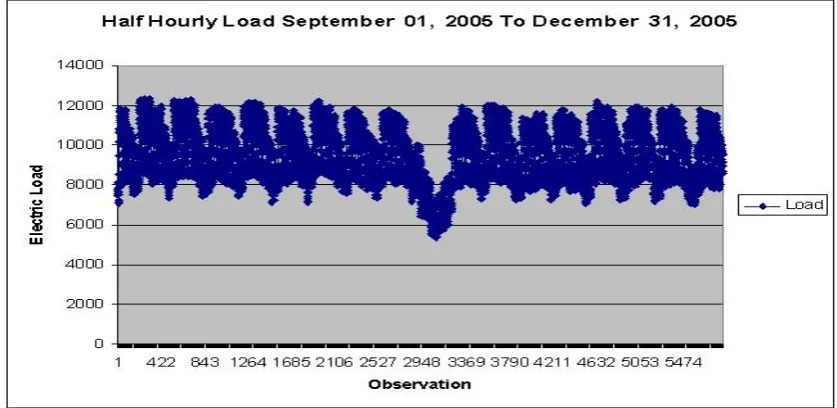
Using Malaysia load data, Mohamed et al. [12][13] showed that the MAPE values using SARIMA and multilayer feed-forward neural network are 0.9774104 and 3.7928802 respectively. The data used are four-month half hourly load demand measured in Megawatts (MW) from September 01, 2005 to December 31, 2005 gathered from Tenaga Nasional Berhad (TNB), Malaysia as illustrated in Figure 1. Using the same data the performances of the hybrid model with selection of the number of hidden nodes for the non linear model are compared. Section 4.1 reports the results obtained from the number of hidden nodes which varies from 1 to 19.
Figure 1. A half Hourly Load from September 01, 2005 to December 31, 2005
4.1 Hidden Nodes of Hybrid Model
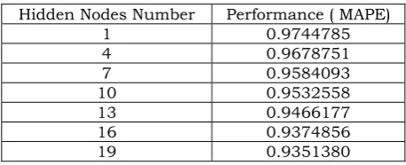
Table 1. The RMSE, MAE and MAPE of the Different Numbers of Hidden Nodes
Hidden Nodes Number Performance ( MAPE)
1 0.9744785 4 0.9678751 7 0.9584093 10 0.9532558 13 0.9466177 16 0.9374856 19 0.9351380
5. CONCLUSIONS
In this paper, we focus on the selection of the appropriate number of hidden nodes in a hybrid model to forecast Malaysia load. Using the mean absolute percentage error (MAPE) as performance measurement, we found that, by using only one hidden node, the hybrid model of Malaysia load performed better than both single models with mean absolute percentage error (MAPE) of less than 1%. Thus, it is concluded that a hybrid model as proposed by this paper will not only improve forecasting performance but will also reduce training time.
REFERENCES
[1]. Bengio, Y., Neural Networks for Speech and sequence recognition, International Thomson Computer Press, 1995.
[2]. Box, G. E. P., Jenkins, G. M. & Reinsel, G. C., Time Series Analysis: Forecasting and Control. Prentice Hall, New Jersey, 1994.
[3]. Brockwell, P. J., & Davis, R. A. Introduction to Time Series and Forecasting, Springer, New York, 1996.
[4]. BuHamra, S., Smaoui, N., & Gabr, M., The Box-Jenkins analysis and neural networks: prediction and time series modeling, Applied Mathematical Modeling, 27, 2003, 805-815. [5]. Chatfield, C., The Analysis of Time Series: An Introduction, Sixth Edition, Chapman & Hall,
New York, 2004.
[6]. Chen, W. H., Shih, J. Y. and Wu, S., Comparison of support vector machines and back propagation neural networks in forecasting the six major Asian stock markets, Int. J. Electronic Finance, 1, 1, 2006, 49-67.
[7]. Eberhart, R. C., Dobbins, R. W., Neural Network PC Tools, A Practice Guide, Academic Press, Inc. London, 1990.
[8]. Fausett, L., Fundamentals of neural networks architecture, algorithms and applications, Prentice Hall, New Jersey, 1994.
[9]. Gonzalez-Romera, E, Jaramillo-Moran, M.A, Carmona-Fernandez, D., Monthly electric energy demand forecasting with neural networks and Fourier series. Energy Conversion and Management, 2008.
[10]. Khoa, N. L. D., Sakakibara, K. and Nishikawa, I., Stock Price Forecasting using Back Propagation Neural Networks with Time and Profit Based Adjusted Weight Factors. SICE-ICASE International Joint Conference, 2006, 5484-5488.
[11]. Makridakis, S., Wheelwright, S. C and Hyndman, R. J., Forecasting: Methods and application. John Willey and Sons, New York, 1998.
[12]. Mohamed, N., Ahmad, M. H., Ismail, Z., and Arshad, K. A., Multilayer Feedforward Neural Network Model and Box-Jenkins Model for seasonal load Forecasting International Journal of Physical Sciences, Ultra Science,20, 2008,767-772.
[13]. Mohamed, N., Ahmad, M. H., Ismail, Z., and Arshad, K. A., A hybrid of artificial neural networks and SARIMA models for load forecasting, International Journal of IT and Knowledge Management, 1, 2008, 179-190.
[16]. Smith, M., Neural Networks for Statistical Modelling, Van Nostrand Reindhold, New York, 1993.
[17]. Tseng, F. -M., Yu, H. -C., and Tzeng, G. -H.., Combining neural network model with seasonal time series ARIMA model, Technological Forecasting & Social Change, 69, 2002, 71-87. [18]. Welstead, S. T., Neural Network and Fuzzy logic applications in C/C++, John Willey and
Sons, Canada, 1994.
[19]. Zhang, G. P., Time series forecasting using a hybrid ARIMA and neural network model, Neurocomputing, 50, 2003, 159-175.