GLOTFELTY, TIMOTHY WILLIAM. Assessing the Impact of Global Air Quality and Climate Interactions in a Changing World using Two Advanced Global Models:
Improvement of Organic Aerosol Formation and Application to Decadal Simulations. (Under the direction of Dr. Yang Zhang).
In this study, two advanced global models are used to simulate future climate policy and air quality scenarios. The Global-through-Urban Weather Research and Forecasting Model with Chemistry (GU-WRF/Chem) is used to simulate the changes in future air quality, climate, deposition, intercontinental transport, and aerosol-cloud interactions following the IPCC AR4 SRES A1B scenario. The Community Earth System Model modified at North Carolina State University (CESM-NCSU) is further developed in this work to include new treatments for the formation of organic aerosol (OA) and its impact on aerosol-climate interactions. Then this modified version of CESM-NCSU is employed to simulate future changes in air quality, climate, deposition, and aerosol-cloud interactions following the IPCC AR5 RCP4.5 and RCP8.5 climate policy scenarios. The objectives of this work are to
improve the representation of OA in CESM-NCSU, evaluate and quantify changes in future air quality and climate using both advanced models, quantify the impact of chemistry on climate following future emission projections using both advanced models, and determine if the use of these advanced models provides additional insights into future climate change and air quality compared to models with less advanced chemistry.
Air quality is degraded in the future following the IPCC AR4 SRES A1B scenario using GU-WRF/Chem with global average increases in maximum 8-hr ozone (O38hr) of 2.5
America and the Arctic. The enhanced aerosol and cloud formation lead to decreases in short-wave radiation reaching the earth’s surface by 1.2 W m-2. However, the use of prescribed sea surface temperatures in GU-WRF/Chem limits the impact of this change in radiative forcing on climate. GU-WRF/Chem shows differences in simulated future climate compared to NCAR’s CCSM3 model with less advanced chemistry, indicating that chemical treatments can have a strong impact on climate change predictions.
The new OA treatments in CESM-NCSU increase simulated levels of oxygenated organic aerosol (OOA) and total organic matter (TOM), but decrease simulated levels of primary organic matter (POM). The reduced POM level decreases the aerosol direct effect of OA, while the increase in OOA increases the aerosol indirect effect of OA within CESM-NCSU. The new OA treatments improve model performance compared to most OA
observations, except hydrocarbon-like aerosol (HOA) that becomes largely underpredicted. The new OA treatments also improve the simulated seasonal patterns of OA and bring the relative contributions of POM and OOA to TOM into better agreement with observations. Overall, CESM-NCSU with the new OA treatments provides an improved representation of the current atmosphere and is thus suitable for future climate simulations.
There are reductions in the future levels of many pollutants following the RCP4.5 and RCP8.5 scenarios simulated by CESM-NCSU, due to reductions in future emissions.
However, there are differences in future O3 projections in both scenarios with a 1.4 ppb
Application to Decadal Simulation
by
Timothy William Glotfelty
A dissertation submitted to the Graduate Faculty of North Carolina State University
in partial fulfillment of the requirements for the degree of
Doctor Philosophy
Marine, Earth, and Atmospheric Sciences
Raleigh, North Carolina 2016
APPROVED BY:
_______________________________ Dr. Yang Zhang
Committee Chair
_______________________________ _______________________________ Dr. Nicholas Meskhidze Dr. Markus Petters
Timothy William Glotfelty was born in Cumberland, Maryland in 1988, and has been a resident of Grantsville, Maryland for the majority of his life. He attended St. Michael’s Catholic Elementary school for kindergarten through sixth grade, after which he transferred to Northern Garrett County Middle school and later attended Northern Garrett County High School to complete his secondary education. During this time period, Timothy had developed an interest in the Earth sciences; especially the weather. While embarking on this educational journey, he enjoyed all manners of science and mathematics classes that provided him with an opportunity to develop a greater understanding and appreciation of the processes that control the Earth and its ecosystems. Upon graduating from Northern Garrett County High School in 2006, he became interested in pursuing a degree in Meteorology.
To accomplish this goal, he enrolled at Frostburg State University in Frostburg, Maryland in fall of 2006 to complete his general education requirements. Later in 2008, he transferred to the Pennsylvania State University (Penn State) in University Park,
Pennsylvania where he completed the majority of his meteorological coursework. During his final summer at Penn State, Timothy undertook an internship at the Pennsylvania Department of Environmental Protection where he developed an interest in air quality modeling and forecasting. After this experience, he began to consider graduate school as a vehicle that would enable him to study air quality and climate change in greater detail. He obtained his B. S. in Meteorology and graduated with high distinction from Penn State in May of 2010.
During the course of his studies at NCSU, he was able to participate in two research
Now that I have reached the capstone of my education, there are several individuals and agencies I would like to like to acknowledge for their guidance and support. I would first like to thank my entire committee including, Drs. Yang Zhang, Nicholas Meskhidze, Markus Petters, Andrew Grieshop, and Anantha Aiyyer for their guidance and scientific input. I would like to especially thank Dr. Yang Zhang for all the opportunities that she has offered and the patience and dedication she has shown in guiding me to be a research scientist in a challenging field. Special thanks are also due to Drs. Jason Ching formerly of the U.S. EPA, Fei Chen of NCAR, and Kiran Alapaty of the U.S. EPA for providing me moral support, real world training, and other necessary skills for my career and the completion of my degree. The inspiration and memories that came from my experiences with them have provided me the motivation to finish my degree and some of the best memories of my Ph. D studies. Thanks are also due to the following individuals who provided support of data necessary for this research including, Drs. Gary Howell and Eric Sills from the High Performance and Grid Computing Center at NCSU. Dr. Prakash Karamchandani of ENVIRON International
Corporation, Dr. David Streets of Argonne National Lab Energy Systems Division, and Drs. Louisa Emmons, Mark Richardson, William C. Skamarock, and Francis Vitt of NCAR.
Information Systems Laboratory, sponsored by the National Science Foundation. MODIS data and CERES data are provided by NASA via http://ladsweb.nasa.gov/data/search.html and http://ceres.larc.nasa.gov/order_data.php, respectively. Other surface network data were downloaded from their respective web sites. AQMEII emissions for CONUS were prepared by U.S. EPA, Environment Canada, Mexican Secretariat of the Environment and Natural Alessandra Balzarini, Research on Energy System (RES), Italy. MEIC emissions for China were provided by Qiang Zhang and Kebin He, Tsinghua University, China.
I am especially grateful for the support of my past and current colleagues at the NCSU Air Quality Forecast Laboratory, including Kai Wang, Jian He, Khairunissa Yahya, Patrick Campbell, Brett Gantt, LeeAnna Young Chapman, Catalina Segura, Ashley Penrod, Ying Chen, Xin Zhang, Changjie Cai, Shuai Zhu, Maslin Gudoshava, Yao-Sheng Chen, Nan Zhang, and many others.
LIST OF TABLES ... ix
LIST OF FIGURES ... xi
LIST OF ACRONYMS ... xxi
CHAPTER 1. INTRODUCTION ... 1
1.1 Background ... 1
1.2 Objectives, Hypothesis, and Proposed Research ... 6
CHAPTER 2. CHANGES IN FUTURE AIR QUALITY, DEPOSITION, AND AEROSOL-CLOUD INTERACTIONS UNDER THE IPCC AR4 SRES A1B SCENARIO USING GU-WRF/CHEM ... 14
2.1 Review of Climate Change Impacts on Air Quality ... 14
2.2 Model Configuration, Evaluation Protocol, and Observational Datasets ... 19
2.2.1 Model Configuration and Inputs... 19
2.2.2 Evaluation Protocol ... 25
2.3 Model Evaluation ... 26
2.3.1 Operational Evaluation ... 26
2.3.2 Climate Trend Comparison ... 31
2.4 Projected Emissions ... 36
2.5 Impact on Air Quality ... 39
2.5.1 Trace Gases... 39
2.5.2 PM2.5 ... 44
2.6 Aerosol-Climate Interactions ... 47
2.7 Deposition ... 49
2.8 Sensitivity Analysis ... 51
2.8.1 Impact of Climate Change on Air Quality ... 51
2.8.2 Impact of Changing Emissions on the Future Climate ... 54
2.9 The Impact of Climate and Emissions on East Asian Intercontinental Transport ... 59
2.9.1 Review of Intercontinental Transport Studies ... 59
2.9.5 The Impact of EAAEs on the Climate System ... 83
2.10 Conclusions ... 87
CHAPTER 3. INCORPORATION OF NEW ORGANIC AEROSOL TREATMENTS IN CESM-NCSU ... 132
3.1 Review of Organic Aerosol Modeling ... 132
3.2 Model Development and Improvements ... 140
3.2.1 Organic Aerosol Treatments in the Standard Version of CESM/CAM5.1 ... 141
3.2.2 The New OA Treatments Implemented into CESM-NCSU ... 143
3.2.2.1 The Volatility Basis Set Approach ... 143
3.2.2.2 Glyoxal and Glyoxal SOA Formation ... 149
3.2.2.3 Organic Vapor – Sulfuric Acid Conucleation ... 150
3.3 Model Configurations and Evaluation Protocols ... 152
3.3.1 Model Setup and Simulation Design ... 152
3.3.2 Available Measurements and Evaluation Protocol ... 157
3.4 Uncertainty and Sensitivity Studies of Parameters within the New OA Treatments .. 161
3.4.1 Sensitivity of Organic Aerosol ... 161
3.4.2 Sensitivity of Aerosol/Climate Interactions ... 172
3.5 Impacts of New OA Treatments and Current Period Evaluation ... 178
3.5.1 Evaluation and Comparison of OC, TC, and TOM ... 178
3.5.2 Evaluation and Comparison of HOA, OOA, and SOA ... 189
3.5.3 Evaluation and Comparison of PM2.5 and PM10 ... 195
3.5.4 Impacts and Evaluation of Aerosol/Climate Interactions ... 197
3.6 World Region OA Comparison ... 200
3.7 Conclusions ... 204
CHAPTER 4. CHANGES IN FUTURE AIR QUALITY, DEPOSITION, AND AEROSOL-CLOUD INTERACTIONS UNDER THE IPCC AR5 RCP SCENARIOS USING CESM-NCSU ... 239
4.2.2 Evaluation and Analysis Protocol ... 252
4.3 Evaluation of Current Climate Periods ... 254
4.3.1 Evaluation of Radiation, Cloud Properties, and Meteorological Parameters ... 254
4.3.2 Evaluation of Trace Gases and Aerosols ... 265
4.3.3 Temporal Evaluation Trace Gases, Aerosol, and Aerosol/Cloud Interactions ... 275
4.4 Projected Trends in Climate, Air Quality, and Aerosol-Cloud Interactions ... 281
4.4.1 Trends in Meteorological, Cloud, and Radiation Parameters ... 281
4.4.2 Trends in Trace Gases ... 288
4.4.3 Trends in Aerosols ... 296
4.4.4 Trends in Chemical Deposition ... 300
4.4.5 Trends in Aerosol-Cloud Interactions ... 303
4.5 Impact of Climate Change on Air Quality ... 305
4.6 Impact of Emission Changes on Aerosol Direct and Indirect Effects ... 309
4.7 Conclusions ... 318
CHAPTER 5. SUMMARY ... 354
5.1 Summary ... 354
5.2 Limitations and Future Work ... 361
Table 1.1 Comparison of Treatments in GU-WRF/Chem, CAM5, and
CESM-NCSU ... 13
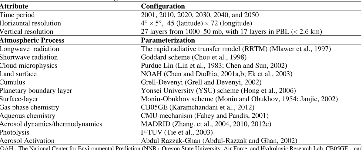
Table 2.1. GU-WRF/Chem Model Configurations ... 96
Table 2.2. Emissions Growth Factors for the Year 2030 ... 97
Table 2.3. Emissions Growth Factors for the Year 2050 ... 98
Table 2.4. Emissions Totals of Anthropogenic Species for Each Simulated Decade ... 99
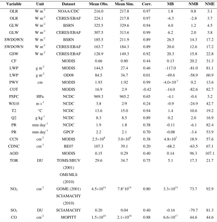
Table 2.5. Model Evaluation Statistics for the Average of the Current Years ... 100
Table 2.6. Correlation of O38hr Response to Climate and Emissions Variables ... 101
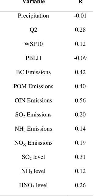
Table 2.7. Correlation of PM2.5 Response to Climate and Emissions Variables ... 102
Table 2.8. Correlation for Sensitivity of O38hr Response to Climate Variables ... 103
Table 2.9. Correlation for Sensitivity of PM2.5 Response to Climate Variables ... 103
Table 3.1. Comparison of Organic Aerosol Modeling Approaches ... 210
Table 3.2. Comparison of VBS Treatments in the Literature. ... 211
Table 3.3. Comparison of Performance Statistics of OA over CONUS. ... 212
Table 3.4. Comparison of Performance Statistics against European EMEP OC Observations. ... 212
Table 3.5. Comparison of Performance Statistics against Z07 & J09. Observations ... 213
Table 3.6. The CESM-NCSU Model Configurations for SOA Modeling. ... 213
Table 3.7. SOA Mass Yields for VOC Precursors (Murphy and Pandis, 2009; Ahmadov et al., 2012) used in this work. ... 214
Table 3.10. List of Datasets for OA, PM, Radiation, and Cloud Evaluation ... 216
Table 3.11. Normalized Mean Bias for OA Sensitivity Simulations ... 217
Table 3.12. Probability of Difference in Simulated Fields from Sensitivity Experiments ... 217
Table 3.13. Probability of Difference in Simulated Fields between the Baseline and New OA Treatments ... 218
Table 3.14. Statistical Performance Comparison of Base_OAC (Base), New OAC (New), and Final_OAC (Final) Simulations. ... 219
Table 3.15. Regional Maximum and Spatial Mean OA levels. ... 220
Table 4.1. List of Datasets for Meteorological, Cloud, and Radiation Evaluation ... 325
Table 4.2. List of Datasets for Chemical Evaluation ... 326
Table 4.3. Performance Statistics of Radiation, Cloud, and Meteorological Variables ... 327
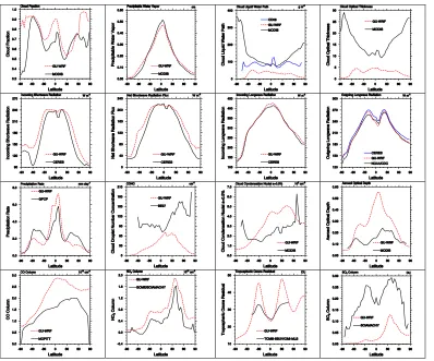
Figure 2.1. The zonal mean profiles of CF, LWP, COT, CCN, PWV, precipitation rate, OLR, AOD, column SO2, column CO, column NO2, and TOR from
GU-WRF/Chem compared against the zonal mean profiles of
observations from the MODIS, MOPITT, GOME, TOMS-SBUV, OMI-MLS, SCIAMACHY, NOAA/CDC, and GPCP satellite and reanalysis
datasets for the average current year period (2001 and 2010). ... 104 Figure 2.2.Spatial distributions of simulated SWDOWN and GLW overlaid with
observations from the BSRN surface network and those of T2, Q2, wind speed at 10-m, and precipitation overlaid with observations from the NCDC surface network for the average current year period (2001 and
2010). The observations are symbolled as circles. ... 105 Figure 2.3. The absolute difference between simulated AOD and MODIS estimated
AOD for the AOC period ... 106 Figure 2.4. A comparison of the variation trends in surface temperature, surface water
vapor, net shortwave radiation at the Earth’s surface, outgoing longwave radiation at the top of the atmosphere, precipitation rate, and surface sulfate concentration between the average current year period (2001 and 2010) and the average future year period (2020, 2030, 2040, and 2050)
for both the CCSM3 and GU-WRF/Chem simulation. ... 107 Figure 2.5. The absolute difference in meteorological, cloud, and radiation variables
from GU-WRF/Chem and CESM1-CAM5 between the AOF and AOC
periods. ... 108 Figure 2.6. The absolute differences in anthropogenic emissions of TNVOC, NOX,
CO, CH4, SO2, NH3, BC, POM, and other unspeciated PM2.5 aerosol
4
AOC periods. ... 110 Figure 2.8. The absolute differences in the CO, NH3, SO2, NO2, O38hr, PAN, OH,
HO2, H2O2, NO3 radical, N2O5, and HNO3 level between the AOF and
AOC time periods. ... 111 Figure 2.9. The absolute differences in average PM2.5 level and its component species
between the AOF and AOC time periods. ... 112 Figure 2.10.Absolute changes in aerosol number concentration, column cloud
condensation nuclei concentration at a supersaturation of 0.5%, column cloud droplet number concentration, cloud liquid water path, cloud optical thickness, aerosol optical depth, incoming shortwave radiation,
and NO2 photolysis rate between the AOF and AOC periods. ... 113
Figure 2.11. The vertical zonal averaged cross section difference in PM2.5 between the
AOF and AOC periods. ... 114 Figure 2.12.Absolute changes in the total deposition flux of O3, total nitrogen, NH3,
HNO3, BC, and Hg between the AOF and AOC periods. ... 115
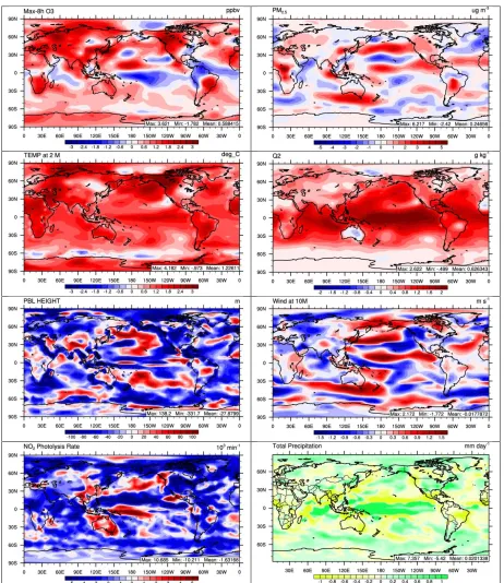
Figure 2.13. Absolute differences in O38hr, PM2.5, T2, Q2, PBLH, WSP10, NO2
photolysis rate, and precipitation between the 2050 climate change only
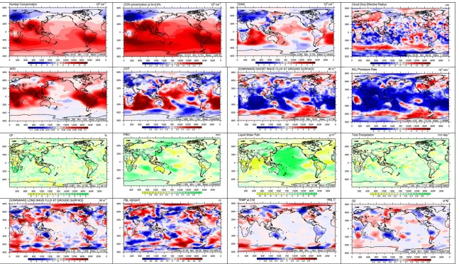
simulation and 2001 ... 116 Figure 2.15. Absolute differences in NUM, CCN, CDNC, Reff, AOD, COT,
SWDOWN, NO2 photolysis rate, CF, PWV, LWP, PR, GLW, PBLH,
T2, and Q2 between the 2050 simulation with projected emissions and
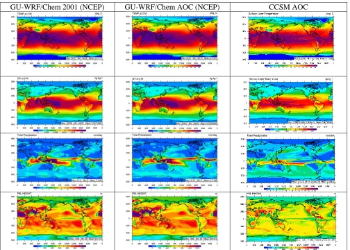
the 2050 simulation without projected emissions ... 117 Figure 2.16. Average spring (MAM) 2-m temperature, 2-m water vapor, precipitation
with the NCEP-FNL data. ... 118 Figure 2.17. Average spring (MAM) 2-m temperature, 2-m water vapor, precipitation
rate, and planetary boundary layer height fields from GU-WRF/Chem simulations of the year 2050 (left), averaged future period consisting of 2020, 2030, 2040, and 2050 (AOF) (center), and the average of the
future period 2015-2054 from CCSM3 initial conditions (right). ... 119 Figure 2.18. Average spring (MAM) 2-m temperature, 2-m water vapor, precipitation
rate, and planetary boundary layer height fields from GU-WRF/Chem simulations of the year 2001 (left), averaged current period consisting of 2001 and 2010 (AOC) (center), and the average of the current period
2000-2014 from CCSM3 initial conditions (right) ... 120 Figure 2.19. The statistically significant differences in T2, Q2, SLP, WSP10,
WSP5500, PR, GSW, OLR, and GLW between MAM 2050 and 2001 that are greater than the variability in the current climate from reanalysis or satellite data (left) and greater than the variability in the current and future climate from CCSM3 (right). The GLW plot in the bottom row of the CCSM3 column was not generated since the CCSM3 GLW data was
not readily available. ... 121 Figure 2.20. The statistically significant differences in T2, Q2, SLP, WSP10,
WSP5500, PR, GSW, OLR, and GLW between MAM AOF and AOC that are greater than the variability in the current climate from reanalysis or satellite data (left) and greater than the variability in the current and future climate from CCSM3 (right). The GLW plot in the bottom row of the CCSM3 column was not generated since the CCSM3 GLW data was
2
carbon, and primary organic carbon. ... 123 Figure 2.21. The time evolution of NO, volatile organic compound, black carbon,
organic carbon, CO, SO2, and NH3 emissions in the GU-WRF/Chem
A1B, RCP6, and RCP8.5 emission scenarios on a global scale. ... 124 Figure 2.22. The time evolution of NO, volatile organic compound, black carbon,
organic carbon, CO, SO2, and NH3 emissions in the GU-WRF/Chem
A1B, RCP6, and RCP8.5 emission scenarios in East Asia. ... 125 Figure 2.23. The average spring (MAM) weather patterns at the surface (top) and
5500 m (bottom) for 2001 and the average current period (left), 2050 and the average future period (right) from the baseline simulations. The surface plots depict the wind vectors from the 10 m wind components and the color scale is based on the sea level pressure. The 5500 m vectors are derived from the wind components interpolated to that
height and the color scale is the magnitude of the wind speed. ... 126 Figure 2.24. The difference in the spring (MAM) maximum 8-hr average surface
ozone mixing ratio (top) and the mid-latitude (24°N to 60°N) meridional averaged vertical cross section of ozone (bottom) between the
simulations with and without EAAEs for the current (2001) and future
(2050 and 2050_CCO) scenarios. ... 127 Figure 2.25. The difference in the spring (MAM) 24-hr average PM2.5 concentration
(top) and the mid-latitude (24°N to 60°N) meridional averaged vertical cross section of PM2.5 (bottom) between the simulations with and
without EAAEs for the current (2001) and future (2050 and 2050_CCO)
total gaseous and particulate mercury (row 4) between the simulations with and without EAAEs for the current (2001) and future (2050)
scenarios. ... 129 Figure 2.27. The difference in the spring (MAM) average cloud condensation nuclei
(CCN), cloud droplet number concentration (CDNC), cloud optical thickness (COT), aerosol optical depth (AOD), downward solar radiation flux (SWDOWN), and the photolysis rate of NO2 (JNO2)
between the simulations with and without EAAEs for the current
(2001), future (2050), and climate change only (2050_CCO) scenario. ... 130 Figure 2.28. The difference in the spring (MAM) average 2 m temperature, planetary
boundary layer height, total precipitation rate, and 10 m wind speed between the simulations with and without EAAEs for current (2001),
future (2050), and climate change only (2050_CCO). ... 131 Figure 3.1. Flow chart that summarizes the differences between the CESM-NCSU
Base organic aerosol treatment and the CESM-NCSU new organic aerosol treatments. Tier 1 illustrates the differences between the Base OA treatments and the New OA treatments, Tier 2 (Green Box)
provides greater details on how the gas-aerosol partitioning is handles in the new OA treatments, and Tier 3 (Dashed Boxes) provides greater details on the partitioning calculations. Light blue boxes indicate VSOA specific calculations, red boxes indicate POM specific calculations, orange boxes indicate glyoxal specific calculations, and brown boxes
indicate SVOA specific calculations. ... 221 Figure 3.2. The absolute difference in the concentration of POM between the New
Figure 3.4. The absolute difference in the concentration of SOA between the New OA
simulation and sensitivity simulations 1-14 from Table 4.3. ... 224 Figure 3.5. The absolute difference in the concentration of SVOA between the New
OA simulation and sensitivity simulations 1-14 from Table 4.3. ... 225 Figure 3.6. The absolute difference in the concentration of TOM between the New
OA simulation and sensitivity simulations 1-14 from Table 4.3. ... 226 Figure 3.7. The zonally-averaged cross sectional absolute differences in the
concentration of OOA, CCN at a supersaturation of 0.5%, cloud droplet number, and particle number between the OA_HVAP_SOA (left), OA_NO_WDEP (center), and OA_Final_Mix (right) simulations and
the New OA simulation. ... 227 Figure 3.8. The absolute differences in AOD, COT, and SWCF between the
OA_HVAP (left), OA_NO_WDEP (center), and OA_Final_Mix (right)
simulations and the New_OA simulations. ... 228 Figure 3.9. The zonally-averaged cross sectional absolute differences in CCN at a
supersaturation of 0.5%, cloud droplet number concentration, and COT between the OA_HI_κ (left) and OA_LOW_κ (right) simulations and
the New OA simulation. ... 229 Figure 3.10. The absolute differences in COT, LWP, and SWCF between the
OA_HI_κ (left) and OA_LOW_κ (right) simulations and the New_OA
simulation. ... 230 Figure 3.11. The zonally-averaged cross sectional differences in particle number
Figure 3.13. The absolute difference in the concentrations of POM, SOA, OOA, TOM, PM2.5, AOD, NUM, CCN, CDNC, COT, SWCF, and FSDS
between the Base_OAC and Final_OAC simulations for the average
current time period. ... 233 Figure 3.14. Scatter plots ofobservations versus simulation results from the averaged
current time period Base_OAC and Final_OAC simulations for OC, TC,
SOA, HOA, OOA, TOA, PM2.5, and PM10. ... 234
Figure 3.15. A comparison of the monthly time series of OC and its components from selected sites in the IMPROVE and EMEP networks and monthly time series of TC and its components from the select sites in the STN
network from the Base_OAC, New_OAC, and Final_OAC simulations. ... 235 Figure 3.16. The relative contribution of simulated OA components to the total
simulated OA and TC concentrations at selected IMPROVE, STN, and EMEP sites from the Base_OAC, New_OA, and Final_OAC
simulations. ... 236 Figure 3.17. The relative contributions of HOA and OOA from selected sites in the
Zhang, Q. et al. (2007) and Jimenez et al. (2009) dataset and the relative contribution of the OA species from the CESM-NCSU Base_OAC,
New_OAC, and Final_OAC simulations. ... 237 Figure 3.18. The relative contributions of ASOA and BSOA from selected sites of the
Lewondowski et al. (2013) dataset and similar relative contributions at these sites from the CESM-NCSU New_OAC and Final_OAC
simulations. ... 238 Figure 4.1. A comparison of the zonal mean profiles for cloud and radiation variables
Figure 4.2. A comparison of the zonal mean profiles for surface meteorological variables and trace gas column mass abundances from the RCP4C, RCP8C, and He et al., (2015a) simulations using CESM-NCSU and available CESM-CMIP5 simulations against satellites/reanalysis
estimates. ... 330 Figure 4.6. The monthly-mean times series of tropospheric PM2.5, PM10, and column
mass abundances of HCHO, NO2, and O3 from the RCP4C and RCP8C
simulations compared against available satellite estimates in the five stratocumulus cloud regions of North America (NAM), South America (SAM), South East Asia (SEA), South Africa (SAF), and Australia
(AUS). ... 334 Figure 4.7. The monthly-mean times series (2001-2010) of AOD, column CCN5,
column CDNC, and SWCF from the RCP4C and RCP8C simulations compared against available satellite estimates in the five stratocumulus
cloud regions of NAM, SAM, SEA, SAF, and AUS. ... 335 Figure 4.9. Absolute differences in precipitation rate between the RCP4C simulation
and GPCP estimates during the four seasons: DJF (a), MAM (b), JJA
(c), and SON (d). ... 337 Figure 4.10. A comparison of the spatial trends in available meteorological, cloud,
and radiation variables between CESM-NCSU and CESM1-CMIP5
simulations under the RCP4.5 scenario. ... 338 Figure 4.11. A comparison of the spatial trends in available meteorological, cloud,
and radiation variables between CESM-NCSU and CESM1-CMIP5
simulations. ... 340 Figure 4.13. Absolute differences in the emissions of AVOC, NO, SO2, NH3, CO,
BVOC, BC, OC, sea-salt, and dust emissions between the RCP8F and
RCP8C simulations. ... 341 Figure 4.14. A comparison of trends in surface concentrations of trace gases predicted
by CESM-NCSU between future and current decades under the RCP4.5
and RCP8.5 scenarios. ... 342 Figure 4.15. Absolute differences in surface total chemical production and net
chemical production of O3, OH, and CO between the current and future
periods under the RCP4.5 and RCP8.5 scenarios. ... 343 Figure 4.16. The changes in NOx/VOC photochemical regimes using the NOy level
indicator (top) and O3/NOy ratio indicator (bottom) following the
RCP4.5 (left) and RCP8.5 (right) scenarios. The blue color indicates a transition from VOC-limited conditions in the current period to NOx
limited conditions in the future period, while the red color indicates a transition from NOx limited conditions during the current period to
VOC-limited conditions during the future period. ... 344 Figure 4.17. A comparison of trends in surface concentrations of aerosol species
predicted by CESM-NCSU between future and current decades under
the RCP4.5 and RCP8.5 scenarios. ... 345 Figure 4.18. A comparison of trends in surface concentrations of PM2.5 and PM10
predicted by CESM-NCSU between future and current decades under
the RCP4.5 and RCP8.5 scenarios. ... 346 Figure 4.19. A comparison of trends in deposition of O3, nitrogen, oxidized sulfur
current decades under the RCP4.5 and RCP8.5 scenarios. ... 347 Figure 4.20. A comparison of trends in CCN5, CDNC, COT, and SWCF predicted by
CESM-NCSU between future and current decades under the RCP4.5
and RCP8.5 scenarios. ... 348 Figure 4.21. Absolute difference in O3, CO, PM2.5, PM10, PM2.5 (no dust), PM10 (no
dust), dust, BSOA, SO42-, and Na+ between the RCP4F_GHGF and
RCP4C simulations. ... 349 Figure 4.22. The absolute difference in the zonal mean vertical cross-section of O3
between the RCP4F_GHGF and RCP4C simulations. ... 350 Figure 4.23. The absolute difference in POM, SVOA, ASOA, NH4+, NO3-, Cl-,
planetary boundary layer height, WSP10, and PR between the
RCP4F_GHGF and RCP4C simulations. ... 351 Figure 4.24. Absolute differences in meteorological, cloud, and radiation variables
between the RCP4F and RCP4F_GHGF CESM-NCSU simulation,
illustrating the impacts of changing emissions. ... 352 Figure 4.25. Absolute differences in clear sky FSDS, Sea Level Pressure, SHX, LHX,
lower troposphere RH, lower troposphere temperature, PRC, and PRL
Acronym Definition
1-D One dimensional
1.5-D One and a half dimensional
3-D Three dimensional
ΔHvap Enthalpy of vaporization
ACCMIP Atmospheric Chemistry and Climate Model Intercomparison Project
AF Africa
AIM Asian-Pacific Integrated Model
ALKH Long chain alkanes
AMS Aerosol mass spectrometer
ANL Argonne National Laboratory
AOC Average of current years
AOD Aerosol optical depth
AOF Average of future years
APIN α-pinene
AQS Air Quality System
AR4 Fourth assessment report
AR5 Fifth assessment report
ASOA Anthropogenic secondary organic aerosol
ASOC Anthropogenic secondary organic carbon
AUS Australia
BC Black carbon
BCTD Black carbon total deposition
BDQA Base de Donnẻes sur la Qualite de I’Air
BE07 Bennartz (2007)
BFM Brute force method
BHM Birmingham, AL
BIR Birkenes, Norway
BPIN β-pinene
Br Bromine
BSOA Biogenic secondary organic aerosol
BSOC Biogenic secondary organic carbon
BSRN Baseline surface radiation network
BVOC Biogenic volatile organic compounds
C* Effective saturation concentration
CAM5 Community Atmosphere Model version 5
CAM-Chem Community Atmosphere Model with Chemistry
CB05 2005 Carbon Bond Mechanism
CB05GE 2005 Carbon Bond Mechanism with global extension
CB6 Version 6 of Carbon Bond Mechanism
CCM Chemistry-Climate model
CCN5 Cloud condensation nuclei at a supersaturation of 0.5%
CDC Climate Diagnostic Center
CDNC Cloud droplet number concentration
CERES Clouds and the Earth’s Radiant Energy System
CESM Community Earth System Model
CESM1 Community Earth System Model version 1
CESM1.2.2 Community Earth System Model version 1.2.2
CESM-NCSU Community Earth System Model modified by the North Carolina State
University
CF Cloud fraction
CFCs Chlorofluorocarbons
CH4 Methane
Cl Chlorine
Cl- Particulate chloride
CMIP5 Coupled Model Intercomparison Project Phase 5
CMU Carnegie Mellon University
CO2 Carbon dioxide
COT Cloud optical thickness
CRI Critical refractive index of water
CTM Chemical transport model
CWP Condensed water path
Dcs Critical diameter for ice crystal autoconversion
EAAE East Asian Anthropogenic Emissions
EaSM Earth System Model
EBAF Energy balanced and filled
EMEP European Monitoring and Evaluation Programme
EFA Anthropogenic emission factors
EFBB Biomass burning emission factors
ELVOCs Extremely low volatility organic compounds
EU Europe
FF Functionalization and fragmentation
FLDS Downwelling long-wave radiation at the Earth’s surface
FLNS Net long-wave radiation at the Earth’s surface
FSDS Downwelling short-wave radiation at the Earth’s surface
FSDSC Clear-sky downwelling short-wave radiation at the Earth’s surface
FSNS Net short-wave radiation at the Earth’s surface
FT Free troposphere
F-TUV Fast Tropospheric Ultraviolet-Visible Model.
GCM General Circulation Model
GEOS/Chem Goddard Earth Observing System model with Chemistry
GHG Greenhouse gases
GHGF Greenhouse gas forcing
GLSOA Organic aerosol from glyoxal
GOME Global Ozone Monitoring Experiment
GPCP Global Precipitation Climatology Project
GRSM Great Smokey Mountains National Park, TN
GSW Net downwelling short-wave radiation flux at the Earth’s surface
GU-WRF/Chem Global-through-Urban Weather Research and Forecasting Model with
Chemistry
GWRF Global Weather Research and Forecasting Model
HE15 He et al. (2015a)
Hg Mercury
HgTD Mercury total deposition
HNO3 Nitric acid
HO2 Hydroperoxyl radical
H2O2 Hydrogen peroxide
HOA Hydrocarbon-like organic aerosol
HTAP Hemispheric Transport of Air Pollution
HUM Humulene
IAT Inorganic aerosol thermodynamics
ICs Initial conditions
IMAGE Integrated Model to Assess the Global Environment
IMN Ion mediated nucleation
IMPROVE Interagency Monitoring of Protected Visual Environments
IPCC Intergovernmental Panel on Climate Change
ISOP Isoprene
ISP Ispra, Italy
ITAP Intercontinental transport of anthropogenic pollution
ITCZ Intertropical convergence zone
IVOCs Intermediate volatility organic compounds
J Nucleation rate
J09 Jimenez et al. (2009)
JFD January, February, and December
JJA June, July, and August
JNO2 Photolysis rate of NO2
KMOE Korean Ministry of the Environment
L13 Lewondowski et al. (2013)
LHX Latent heat flux
LIM Limonene
LOWR Lostwood Wildlife Refuge, ND
LTRH Lower troposphere relative humidity
LTT Lower troposphere temperature
LWCF Long-wave cloud forcing
LWP Liquid water path
MADE Modal Aerosol Dynamics Model for Europe
MAM3 3 mode Modal Aerosol Model
MAM7 7 mode Modal Aerosol Model
MB Mean bias
MBO 2-Methyl-3-buten-2-ol
MEGAN Model of Emissions of Gases and Aerosols from Nature
MEPC Ministry of Environmental Protection in China
MLS Microwave Limb Sounder
MODIS Moderate Resolution Imaging Spectroradiometer
MOPITT Measurements Of Pollution In The Troposphere
MOZART-4 Model for Ozone and related chemical Tracers version 4
Na+ Particulate sodium
NAM North America
NAP Naphthalene
NCAR National Center for Atmospheric Research
NCDC National Climatic Data Center
NCEP-FNL National Centers for Environmental Prediction Final Operational Reanalysis
NCP Net chemical production
ND Nitrogen deposition
NH Northern hemisphere
NHIR Northern hemisphere industrial regions
NH3 Ammonia
NME Normalized mean error
NO Nitrogen oxide
NO2 Nitrogen dioxide
NO3
-Particulate nitrate
NO3 Nitrate radical
NOx Nitrogen oxides
NOy Reactive nitrogen
N2O Nitrous oxide
N2O5 Dinitrogen pentoxide
NOAA National Oceanic and Atmospheric Administration
NOAH The National Center for Environmental Prediction (NNR), Oregon State
University, Air Force, and Hydrologic Research Lab
NUM Column particle number concentration
O1D Singlet oxygen
O2 Molecular oxygen
O3 Ozone
O38hr Maximum eight hour ozone
OA Organic aerosol
OC Organic carbon
OCI Ocimine
OD08 O’dell et al. (2008)
OLE Terminal olefins
OLR Outgoing long-wave radiation
OM Organic matter
OMI Ozone Monitoring Instrument
ON Oxidized nitrogen
OOA Oxygenated organic aerosol
OPOM Oxidized primary organic matter
OSR Outgoing short-wave radiation
PAH Polycyclic aromatic hydrocarbons
PAMS Photochemical Assessment Monitoring Stations
PAN Peroxyacetyl nitrate
PBL Planetary boundary layer
PBLH Planetary boundary layer height
PHO Phoenix, AZ
PM2.5 Particulate Matter with diameter less than or equal to 2.5 μm
PM10 Particulate Matter with diameter less than or equal to 10.0 μm
POC Primary organic carbon
POM Primary organic matter
PSFC Atmospheric surface pressure
PR Precipitation rate
PRC Convective precipitation rate
Q2 2m Water vapor mixing ratio
R Pearson’s correlation coefficient
RACM Regional Atmospheric Chemistry Mechanism
RCP Representative Concentration Pathways
RCP2.6 RCP pathway with radiative forcing of 2.6 W m-2 by 2100
RCP4.5 RCP pathway with radiative forcing stabilizing at 4.5 W m-2 by 2100
RCP6 RCP pathway with radiative forcing stabilizing at 6.0 W m-2 by 2100
RCP8,5 RCP pathway with radiative forcing of 8.5 W m-2 by 2100
Reff Column average cloud drop effective radius
RESTOA Net radiation at the top of the atmosphere
RHMINL Threshold relative humidity for low level cloud formation
RMSE Root mean square error
RN Reduced nitrogen
RRTM Rapid radiative transfer model
RTP Research Triangle Park, NC
S08 Shrivastava et al. (2008)
SA South Asia
SAF Southern Africa
SAM South America
SCIAMACHY SCanning Imaging Absorption SpectroMeter for Atmospheric CHartographY
SEA Southeast Asia
SHX Sensible heat flux
SLP Sea level pressure
SO2 Sulfur dioxide
SO4
2-Particulate sulfate
SOx Oxidized sulfur
SOA Secondary organic aerosol
SOAG Gases that form SOA
SON September, October, and November
SRES Special Report on Emissions Scenarios
SSPs Shared socioeconomic pathways
SSTs Sea-surface temperatures
STE Stratosphere-Troposphere exchange
STN Speciation Trend Network
SVOA Semi-volatile organic aerosol
SVOCs Semi-volatile organic compounds
SWCF Short-wave cloud forcing
SWDOWN Downwelling short-wave radiation flux at the Earth’s surface
T2 2-m Temperature
TAQMN Taiwan Air Quality Monitoring Network
TC Total carbon
TCO Tropospheric carbon monoxide
TND Total nitrogen deposition
TNO2 Tropospheric nitrogen dioxide
TNTD Total nitrogen total deposition
TNVOC Total non-methane volatile organic compounds
TOL Toluene
TOM Total organic matter
TOMS Total Ozone Mapping Spectrometer
TOR Tropospheric ozone residual
UD Urban downwind
VBS Volatility basis set
VMRS Volume mixing ratios
VOC Volatile organic compounds
VSOA SOA from volatile organic compounds
WACCM Whole Atmosphere Community Climate Model
WSP10 10-m Wind speed
WSP5500 5500-m Wind speed
XYL Xylene
YSU Yonsei University
CHAPTER 1. INTRODUCTION 1.1 Background
Two of the most important issues facing the scientific community during the current era are the prospect of global climate change and air pollution. As the global population increases, there is an increasing demand for energy and food resources. The by-products of producing these resources are the release of trace gases and aerosol particles into the atmosphere. Some of these gases known as the greenhouse gases (GHGs) (e.g., CO2, CH4,
and N2O) perturb the earth’s radiation balance. With the exception of CH4, other gases and
particles are typically referred to in the literature as short-lived climate pollutants (e.g., ozone (O3) and particles with aerodynamic diameter less than or equal to 2.5 µm (PM2.5)), both
perturb the earth’s radiation balance and are hazardous to human and ecosystem health (Pierrehumbert, 2014). Hence, understanding the impact of future air quality/ climate interactions is necessary for policy makers to develop the most optimum climate mitigation and air pollution control strategies.
growth, technology change, and energy generation (IPCC, 2001). However, one key limitation of the IPCC AR4 SRES scenarios is that they do not reflect changes from future emission control policies (IPCC, 2007). Thus, as part of the IPCC AR5 the Representative Concentration Pathway (RCP), scenarios were developed. These scenarios are also based on socio-economic factors such as population and economic growth, but they assume major changes in energy generation technologies as a result of climate policy implementation, with a special emphasis on Carbon Capture and Storage (CCS) technologies that help to mitigate the emission of greenhouse gases (van Vuuren et al., 2011b). In addition to major changes in energy generation technologies, these scenarios include the implementation of current and proposed air pollution control measures and the implementation of such control measures in developing countries when the income gap between these countries and developing world decreases (van Vuuren et al., 2011b).
Another key element of future air quality/ climate interaction studies is the modeling tool. Traditionally, future air quality studies used models with offline-coupled architecture (Jacob and Winner, 2009). In this architecture, the climate scenario information (e.g., GHG levels and prescribed aerosol levels) are used to drive an atmospheric General Circulation Model (GCM). GCMs are global weather models that simulate the atmosphere’s dynamical and physical processes and that have usually been calibrated for long-term climate
levels and aerosols based on future climate GCM meteorology and projected future emissions. Future climate and air quality studies using this offline architecture are simple ways to estimate future air quality given a specific scenario. However, they are limited as they cannot simulate air quality/climate interactions, such as direct radiative forcing from prognostic changes in O3 and aerosols, and the aerosol indirect effects on clouds.
To overcome these limitations, online-coupled GCM-CTM models, also known as Chemistry-Climate Models (CCMs), have been developed (Eyring et al., 2005; 2006). These models simulate chemical species and metrological processes within the same model
use and models with each of these configurations have taken part in the Atmospheric Chemistry and Climate Model Intercomparison Project (ACCMIP). ACCMIP compared an ensemble of simulated fields from various global air quality models predicting historical and future air quality following the IPCC AR5 RCP scenarios (Lamarque et al., 2013).
Despite the availability of many modeling tools for future air quality/climate studies, these studies can be limited by the use of simplistic parameterizations for meteorological and chemical processes. For example, the recently-developed Community Earth System Model (CESM) (Hurrell et al., 2013) and the CCM version known as the Community Atmosphere Model with Chemistry (CAM-Chem) (Lamarque et al., 2012) do not consider the role of inorganic aerosol thermodynamics (IAT). IAT is a fairly imperative process to be considered as part of air quality studies because an IAT module is necessary to accurately simulate the formation of aerosol ammonium (NH4+) and nitrate (NO3-) and the sea-salt acidification
process. These processes are neglected in even the most advanced aerosol module in the officially-released version of CESM from NCAR (Liu et al., 2012). This omission may be somewhat justified based on the application of the CESM model as the abundance of sulfate (SO42-) is generally larger than other inorganic aerosol components over the Northern
Hemisphere based on aerosol mass spectrometer (AMS) measurements (Zhang et al., 2007; Jimenez et al., 2009). However, this lack of IAT means that certain important scientific questions cannot be addressed, such as, how much NO3- will compensate SO42- from future
sulfur dioxide (SO2) emission reductions? (Fiore et al., 2012). Nonetheless, this limitation
There are similar or perhaps larger issues regarding the formation of organic aerosols (OA) within CCMs. OA is a major component of total aerosol comprising roughly (18-70%) (Zhang et al., 2007; Jimenez et al., 2009). Typically OA is treated in global models as two separate classes of aerosol. The first is primary organic matter (POM) that is emitted directly into the atmosphere via combustion and behaves similar to a tracer compound. The second is secondary organic aerosol (SOA) that is formed in the atmosphere through the condensation and partitioning of certain low volatility organic vapors. This two species treatment is typical in global models such as the 3 mode or 7 mode Modal Aerosol Model (MAM3 or MAM7) within CESM (Liu et al., 2012). However, there are many CCMs that partially or entirely neglect the formation of SOA (Jacob and Winner, 2009; Fiore et al., 2012). These
representations of OA in CCMs are problematic in light of the scientific progress regarding OA formation within the last decade. OA research has shown that POM is volatile and thus a significant portion of it evaporates into organic vapors (Lipsky and Robinson, 2006;
aerosol components and the increase of biogenic volatile organic compound (BVOC) emissions (Tagaris et al., 2007; Heald et al., 2008).
1.2 Objectives, Hypothesis, and Proposed Research
The overall objectives of my Ph. D research are to quantify changes in future air quality and air quality/climate interactions by the year 2050 using two advanced global air quality models. These models include the Global through Urban Weather Research and Forecasting Model with Chemistry (GU-WRF/Chem) (Zhang et al., 2012b) and the
Community Earth System Model developed at the North Carolina State University (CESM-NCSU) (He et al., 2015a, b). The GU-WRF/Chem model is roughly equivalent to a GCM-CTM architecture CCM, although it has not undergone the extensive calibrations needed for long-term climate simulations. CESM-NCSU is an EaSM that is configured in a CCM mode. The specific objectives of this research are:
(1) To implement, evaluate, and perform sensitivity analysis on new OA treatments in the CESM-NCSU model;
(2) To evaluate the ability of the GU-WRF/Chem and CESM-NCSU models to represent the current atmosphere;
(3) To quantify changes in future air quality between the current time period and the mid-21st Century, following the IPCC AR4 SRES A1B and IPCC AR5 RCP4.5/RCP8.5 scenarios using the GU-WRF/Chem and CESM-NCSU models, respectively; (4) To determine the impact of future emission changes on climate and the impact of
IPCC AR5 RCP4.5 scenarios using the GU-WRF/Chem and CESM-NCSU models, respectively;
The ultimate goal of this research is to demonstrate the importance of using advanced modeling tools for doing future air quality and air quality/climate interaction studies and provide quantifications of these future climate scenarios to the scientific community so that the results are available to be compared with other studies or used as part of future emission control and climate mitigation strategies. The main hypothesis of this work is that chemical processes especially those related to aerosol are important for climate change predictions and conversely the changes in climate are important for predicting future air quality. Several science and policy-related questions will be addressed. For example, how will changing global climate and emissions impact global air quality? What are their relative contributions? How will intercontinental transport of pollution change in the future and what factors
dominate those changes? Will updated treatments for OA improve a climate model’s ability to predict OA and subsequently improve the accuracy of predicted aerosol, cloud properties, and radiative forcing through the aerosol direct and indirect effects? How will these
processes be affected by future changes in biogenic emissions and changes in oxidant levels? How much biogenic SOA is controllable by controlling anthropogenic emissions?
due to more advanced model representations of land use, sea-surface temperatures, and sea ice. However, CESM-CAM5 uses relatively simplistic treatments for many chemical processes except for the gas-phase chemical mechanism that can be configured to be either simple or complex based on the user’s needs. However, all climate applications of CESM-CAM5 thus far used the simple chemical mechanism. This facilitated a need to develop CESM-NCSU that combines advanced chemical treatments similar to those found in GU-WRF/Chem for the superior climate modeling of CESM-CAM5. This development also included improving processes that are treated in a simplistic way in GU-WRF/Chem, such as new particle formation (He and Zhang, 2014), aerosol activation (Gantt et al., 2014), and organic aerosol formation (this work, and also in Glotfelty et al., 2016a).
GU-WRF/Chem 2050 simulation indicates the changes in future climate caused by future emissions changes. GU-WRF/Chem is an older model with an online-coupled GCM-CTM style CCM structure similar to many of the classic chemistry-climate studies. Since GU-WRF/Chem is comparable to models that took part in phase three of the IPCC Coupled Model Intercomparison Project (CMIP3), this study follows the older IPCC AR4 SRES A1B scenario. Trends in GU-WRF/Chem simulated fields are compared against those predicted by the Community Climate System Model version 3 (CCSM3) that also follows this scenario. Since CCSM3 does not simulate prognostic chemistry, this comparison illustrates the importance of using online-coupled CCM structure.
GU-WRF/Chem is also used to investigate the current and future role of ITAP from East Asia. This is achieved by conducting additional 2001and 2050 simulations with East Asian Anthropogenic Emissions (EAAE) removed. This will quantify how ITAP will change under this scenario, determine what factors dominate these changes, and also allow for the impact of EAAEs on biogenic SOA (BSOA) levels to be investigated.
Although GU-WRF/Chem has advanced parameterizations to simulate atmospheric chemistry, the model is limited by a number of factors discussed in Chapter 2.
WRF/Chem is designed primarily for short term air quality simulations. As a result, GU-WRF/Chem has static land use changes between current and future periods and sea ice/se surface temperatures are prescribed. Additionally, GU-WRF/Chem’s transport scheme is not positive definite allowing to errors in the transport of chemical tracers. Due to these
gas-phase chemistry and still contains simplified representations of inorganic and organic aerosol formation. These limitations have been overcome due to modifications made by NCSU, leading to a new CESM-NCSU model (He and Zhang, 2014; Gantt et al., 2014) that is further developed and used for decadal climate simulations in the second portion of this work.
The second portion of this research focuses on further development, evaluation, and application of the CESM-NCSU model. In order to further develop CESM-NCSU, new treatments for OA are implemented into the model. These include (1) a VBS framework treatment for the simulation of POM volatility and SOA formation, including OA aerosol formed from semi-volatile organic compounds (SVOCs) generated from POM evaporation, (2) the addition of an OA generation pathway from glyoxal, and (3) the addition of a treatment for the conucleation of organic vapors and sulfuric acid. These new treatments allow for a more detailed and potentially more realistic simulation of OA in the model. Simulations of the current atmosphere with these updated treatments are evaluated under current climate conditions and compared against current climate simulations of the baseline model to determine differences and improvements in model performance. Sensitivity analysis is also carried out by adjusting various aspects of the new OA treatments to estimate the uncertainties associated with the new OA treatments.
finalized OA treatment is discussed in Chapter 4. The procedure for this study is similar to the GU-WRF/Chem study but with a future time period focused closer to 2050 on a decadal scale (2046-2055). The current climate period (2046-2055) is evaluated using emissions of both scenarios and this evaluation is compared against a CESM-NCSU simulation using more detailed emissions to determine potential limitations of the RCP emissions inventory. Furthermore, this study also focuses on the impact of climate change on future air quality and the impact of future emission changes on climate following the RCP4.5 scenario. This is performed by comparing the future and current period RCP4.5 simulations against a sensitivity simulation of the 2046-2050 period using the current era RCP emissions. Future trends under both RCP scenarios are compared between CESM-NCSU and a version of CESM that uses highly-simplified chemistry to again illustrate the impact of the more advanced chemical treatments on future climate projections.
This work differs from previous studies by examining not only the impact of
The research compiled here is a collection of scientific manuscripts that are either current published or will be part of future publications, The majority of the GU-WRF/Chem climate application in Chapter 2 is part of a published manuscript (Glotfelty et al., 2016b), except for Section 2.9 that has been published as a standalone article (Glotfelty et al., 2014). Chapter 3, which focuses on the development of OA in CESM-NCSU, is currently being prepared for publication (Glotfelty et al., 2016a). Lastly, Chapter 4 is currently being revised into a two part publication (Glotfelty et al., 2016c, d), with part 1 focusing on the
Table 1.1 Comparison of Treatments in GU-WRF/Chem, CESM-CAM5, and CESM-NCSU
Model GU-WRF/Chem CESM-CAM5 CESM-NCSU
Architecture CCM EaSM EaSM
Land Use Static Dynamic Vegetation Dynamic Vegetation
Sea-Surface Temperatures Prescribed Prognostic Prognostic
Sea Ice Prescribed Prognostic Prognostic
Gas-phase Chemistry Advanced Simple/Advanceda Advanced
Aqueous Chemistry Advanced Simple Simple
New Particle Formation Simple Simple Advanced
Inorganic Aerosol Advanced Simple Advanced
Organic Aerosol Simple Simple Advanced
Aerosol Activation Simple Simple Advanced
References Z12bb H13c HZ14d, G14e, G16af
a
CHAPTER 2. CHANGES IN FUTURE AIR QUALITY, DEPOSITION, AND AEROSOL-CLOUD INTERACTIONS UNDER THE IPCC AR4 SRES A1B
SCENARIO USING GU-WRF/CHEM 2.1 Review of Climate Change Impacts on Air Quality
As the global population increases and industrialization grows in a changing climate, it is critical that governmental agencies account for changes in global air quality when forming successful climate change and air pollution mitigation strategies. A warmer and more humid climate with an increased abundance of atmospheric CO2 is generally expected
in the future and this has important ramifications for global air quality (Vautard and Hauglaustaine, 2007; Jacob and Winner, 2009; Weaver et al., 2009; Jacobson and Streets, 2009; Fiore et al., 2012). In addition, several studies have indicated that there is a higher probability of heat waves and air pollution episodes in the future due to increased
stagnation. This results from a poleward shift in stormtracks and a general decrease in the frequency of mid-latitude cyclones (Mickley et al., 2004; Yin, 2005; Vautard and
(Fang et al., 2011). However, there may be a potential increase in boundary layer export due to increases in convection (Zeng et al., 2008).
The warmer and wetter climate is expected to reduce the background ozone (O3) level
in regions with low NOx levels, while increasing O3 level in more polluted regions
(Hauglaustaine et al., 2005; Liao et al., 2006; Murazaki and Hess, 2006; Stevenson et al., 2006; Hedegaard et al., 2008; Wu et al., 2008; Zeng et al., 2008; Jacob and Winner, 2009; Fiore et al., 2012; Doherty et al., 2013). The decreased background concentrations are the result of increased water vapor which reduces the lifetime of O3 by removing O1D to form
the hydroxyl radical (OH), which in turn can destroy O3 through HOx reactions (Doherty et
al., 2013). However, this general reduction in O3 is compensated by increases in
troposphere/stratosphere exchange due to strengthening of the Brewer-Dobson circulation expected in a warmer, CO2 rich climate (Hauglaustaine et al., 2005; Buchart et al., 2010;
Fiore et al., 2012). The O3 level is increased in polluted regions due to higher temperatures
leading to higher O3 formation rates, increases in emissions of biogenic VOCs, and
increased decomposition of peroxyacetyl nitrate (PAN), as well as reduced ventilation from source regions (Hedegaard et al., 2008; Liao et al., 2006; Wu et al., 2008; Zeng et al., 2008). In addition to changes in mean O3, there is a tendency for increases in the 95th percentile O3
(Weaver et al., 2009; Langner et al., 2012), even in cases where the mean O3 level decreases
(Langner et al., 2012). Similarly, the impact of climate change alone results in over half the eastern U.S. exceeding a maximum 8-hr O3 level of 75 ppb assuming emissions remain the
pollution episodes which have been estimated to increase in duration from 2 to 3-4 days with increased pollution levels of 5-10% in the U.S. (Mickley et al., 2004).
The impact of a changing climate on aerosols is less certain than that of O3 because it
is comprised of many different species that respond differently to perturbations in climate and emissions. The impact of future wet deposition is uncertain as it has been shown to both increase in the future resulting in decreases in PM2.5 (Liao et al., 2006) and also potentially
decrease globally due to reductions in annual large scale precipitation over land and seasonal changes in precipitation (Fang et al., 2011). Generally, precipitation changes are variable between models and the impacts are more regional, as wet deposition of soluble aerosols is not strongly dependent on global changes in precipitation (Fiore et al., 2012). PM2.5 is also highly correlated with meteorological phenomena, such as the passage of cold
fronts, but the projected increased stagnation in the future is not expected to induce a climate change penalty of more than 0.5 μg m-3
(Tai et al., 2012).
Changes in climate and emissions are also expected to affect PM2.5 speciation. The
warmer and wetter climate is generally more oxidant rich which results in greater
conversion of SO2 to sulfate (Unger et al., 2006; Hedegaard et al., 2008; Jacob and Winner,
2009). This increased oxidation capacity along with potential increases in biogenic volatile organic compounds (VOCs) will lead to greater formation of both biogenic and
projection. Under the Intergovernmental Panel on Climate Change (IPCC) Fourth
Assessment Report (AR4) Special Report on Emissions Scenarios (SRES) A1B scenario, the decreases by 2100 in emissions of sulfate, nitrate, and ammonium precursors are larger than those of primary organic matter (POM). This coupled with an increase in SOA may lead to organic matter (OM) as a dominant PM2.5 species (Tagaris et al., 2007). It is also
possible in certain regions that declining SO2 emissions and increasing NH3 emissions may
lead to nitrate formation that is equivalent to current PM2.5 levels (Fiore et al., 2012). This
changing speciation over time may lead to variation in climate forcing. The work of Levy et al. (2008) showed that in 2030 following the SRES A1B scenario the climate is only weakly dependent on short lived climate forcers (sulfate, OM, black carbon (BC), O3) due to
compensating effects, but by 2100 enhanced BC emissions of 100% and a roughly 60% decrease in SO2 emissions will contribute 1.5-2.0°C to global warming. This is a result of an
enhanced warming effect from BC and a reduced cooling effect from sulfate (Levy et al., 2008). There may also be potentially large feedbacks to natural emissions of PM2.5
including sea-salt, mineral dust, and wildfires (Jacob and Winner, 2009; Fiore et al., 2012). Changes in future air quality will also have consequences on ecosystem health. O3
deposition inhibits photosynthesis, damages plant cells, and has been shown to reduce both net primary productivity and carbon sequestration (Felzer et al., 2004). O3 deposition is
expected to increase due to an increase in the leaf area of broadleaf forests (Wu et al., 2012). However, these changes are uncertain as O3 deposition can offset the CO2 fertilization effect
(Felzer et al., 2004). Plant damage from O3 deposition may also have an indirect effect on
impact of O3 on vegetation is also dependent upon emission scenario. Large increases in O3
are to be expected under most of the IPCC AR4 SRES scenarios, making it difficult to achieve standards for crop damage and leading to speculation of possible agricultural concerns in the future (Prather et al., 2003). In contrast, the Representative Concentration Pathway (RCP) scenarios, from the IPCC Fifth Assessment Report (AR5), produce surface level O3 improvements in all but the RCP8.5 scenario compared to present day (Lamarque
et al., 2011, Young et al., 2013; Kim et al., 2015). However, under both types of scenarios nitrogen deposition is expected to increase (Dentener et al., 2006; Lamarque et al., 2011) due to increases in reactive nitrogen (NOy) and NH3 under the SRES scenarios and from
increases in NH3 that compensate losses of NOy under the RCP scenarios. This may result in
ecosystem changes, as 10.1% of natural terrestrial ecosystems are already exposed to nitrogen deposition higher than the critical load estimated to impact sensitive ecosystems (Dentener et al., 2006).
In this work, the Global-through-Urban Weather Research and Forecasting Model with Chemistry (GU-WRF/Chem) is employed to study the impact of climate change and emissions on global air quality under the IPCC AR4 SRES A1B emission scenario. The total impacts, as well as the separate contributions from changing emissions and climate, are investigated. The changes in ambient concentrations, deposition, and the impacts of
chemical transport models. However, this complexity comes at the cost of higher computational resource requirements.
2.2 Model Configuration, Evaluation Protocol, and Observational Datasets 2.2.1 Model Configuration and Inputs
GU-WRF/Chem (Zhang et al., 2012b) is an online-coupled model capable of
simulating the interactions and feedbacks between the chemical and physical processes in the atmosphere. It is a hybrid model generated by replacing the WRF model in the National Oceanic and Atmospheric Association (NOAA)’s mesoscale WRF/Chem with the National Center for Atmospheric Research (NCAR)’s global WRF (GWRF) and then improving several model treatments for their applications on hemispheric to global scales. These improvements include online dust and BVOC emissions, gas-phase chemistry, a photolytic rate scheme, aerosol chemistry and microphysics, and aerosol-cloud interactions. Like GWRF and mesoscale WRF/Chem, GU-WRF/Chem has many different parameterizations for various atmospheric processes occurring on spatial and temporal scales smaller than those that can be resolved explicitly by the model. Table 2.1 contains a list of the chemistry and physics options used and the configuration of the simulations.
Gas-Phase chemistry in GU-WRF/Chem is simulated with the carbon bond
mechanism with global extension (CB05GE) (Karamchandani et al., 2012), that simulates tropospheric chemistry as well as chemistry of the upper troposphere and stratosphere, chemistry of the marine boundary layer, mercury (Hg) chemistry (i.e., elemental (gas) and divalent (gas+aerosol) Hg), and Arctic chemistry. This is done through stratospheric
Cl and 11 Br species, heterogeneous reactions on cloud and aerosol particles, and reactions on polar stratospheric clouds all listed in Karamchandani et al. (2012) Tables 1-5. Aerosol chemistry is simulated using the WRF/Chem coupled Model of Aerosol, Dynamics, Reaction, Ionization, and Dissolution MADRID (Zhang. et al., 2004, 2010, 2012c). that simulates all major aerosol processes including inorganic aerosol thermodynamic equilibrium simulated based on version 1.7 of ISORROPIA (Nenes et al., 1998), nucleation, gas-to-particle mass transfer, condensation, coagulation, and the formation of 25 SOA species from anthropogenic (e.g., toluene and xylene) and biogenic (e.g., isoprene, monoterpene, and sesquiterpene) precursors.
Aerosol direct and indirect effects are simulated in GU-WRF/Chem. Aerosol radiative forcing is calculated based on Mie theory using the Goddard shortwave radiation scheme (Chou et al., 1998). Aerosol indirect effects in GU-WRF/Chem are only treated for large scale resolved clouds. Cloud condensation nuclei are determined based on Kohler theory calculated as a function of aerosol number concentrations and updraft velocity
following the aerosol activation parameterization of Abdul-Razzak and Ghan (2002). Cloud droplet number concentrations (CDNC) are predicted based on major cloud processes including aerosol activation, collision/coalescence, collection by rain drops, snow, and ice crystals, formation of ice crystals thru freezing, and advection as part of the Ghan et al. (1997) parameterization that was incorporated into the existing Purdue Lin cloud
to the Goddard shortwave radiation scheme. More details on the chemical and aerosol-cloud interactions are discussed in Zhang et al. (2012b) and references therein.
GU-WRF/Chem simulations are conducted for a period of six years, with two current years (2001 and 2010) and four future years (2020, 2030, 2040, and 2050). This limited subset of years is used because each year represents a different stage of climate forcing and emissions changes, thus some of the decade to decade variability can be captured within the computational constraints. The initial meteorology and chemical conditions for O3, N2O, and
CH4 come from the Community Climate System Model version 3 (CCSM3) SRESA1B data
set. Other chemical initial conditions for gas species with moderate lifetimes not found in the CCSM dataset (e.g., SO2, PAN, and H2O2) are generated from the Goddard Earth Observing
System Model with Chemistry v7-04-12-Run0
(http://wiki.seas.harvard.edu/geos-chem/index.php/GEOS-Chem_v7-04-12). Short-lived radical gas species (e.g., OH and NO3)
future air quality and the 2050 simulation with projected emissions to examine the impact of changing emissions on the future climate.
The boreal spring months (March, April, and May (MAM)) of 2001 and 2050 during which ITAP is the strongest for the Trans-Pacific region are selected to study the role of intercontinental transport of east Asian air pollutants and their impacts on the U.S. and global air quality and climate. Simulations under different emission and climate scenarios for MAM 2001 and 2050 are conducted and compared to those of the MAM 2001 and 2050 simulations as part of the aforementioned multi-year simulations. The suite of model simulations conducted includes three baseline simulations with EAAEs from the multi-year simulations during MAM: 2001 with current climate conditions and emissions, 2050 with projected climate change and emissions, and 2050 with projected climate change only
years, although some degrees of internal model variability will affect the results. Unlike the 20% reductions of anthropogenic emissions used in other studies (discussed in Section 2.9.1), all Asian anthropogenic emissions are zeroed out in the sensitivity simulations in this work to estimate the maximum possible impacts of EAAEs on global air quality and climate. This will lead to significant nonlinear impacts on O3 and fine particle formation but accounting for
these processes is necessary to quantify the impact that East Asia has on the global chemical/climate system and to understand how this impact will change in response to changing climate and emissions.
The meteorological initial conditions as well as the sea surface temperatures (SSTs) for the non-evaluation simulations are 10 year averages of the CCSM3 data that are centered about each GU-WRF/Chem simulation year (e.g., the year 2030 is initialized with the
average of 2025-2034 from the CCSM3 data), with the exception of 2001 which is initialized with the 5 year period 2000-2004 since the CCSM3 simulation started at the year 2000. The meteorology and the SSTs are reinitialized every month. This is especially important as the model uses static SSTs, which need to be reinitialized in order for the annual variation in SSTs to be represented. The chemical species in the model are reinitialized every 3 months. This allows for a mostly continuous chemistry simulation but prevents excess buildup of pollutants near the top of the model and near the polar singularities that can occur due to the lack of a positive-definite advection scheme in the model. This type of reinitialization
WRF/Chem on which GU-WRF/Chem is based that employed reinitialization in 2 day intervals (Yahya et al., 2014; 2015).
The base anthropogenic emission inventory for the year 2001 has been provided in Table 2 of Zhang et al. (2012b). The natural emissions of biogenic volatile organic
compounds (BVOCs), sea-salt, and dust are calculated online. The BVOCs are generated from the Model of Emissions of Gases and Aerosols from Nature (MEGAN) version 2 (Guenther et al., 2006), sea-salt is calculated using the formulation of Gong et al. (1997) with a correction for the smaller sea-salt particles from O’Dowd et al. (1997), and dust is
generated from the scheme of Shaw (2008) with the modifications of Zhang et al. (2012b). Future emissions projections are based on the IPCC AR4 A1B scenario, which is a scenario of increasing economic and population growth that peaks in the mid-21st century and declines thereafter, with a focus on balanced energy sources (IPCC,2001). The anthropogenic
2.2.2 Evaluation Protocol
The model’s performance with regards to meteorology and chemistry is evaluated for current years using a combination of satellite, global surface networks, and reanalysis data. The evaluation p