Approximate analysis of a multi-class queue with class-dependent window-flow control

(1)

Class-Dependent Window-Flow Control"

Raif

o.

Onvural

BNR

Network Intelligence Division RTP, NC 27709-3478

Center for Communications and Signal Processing North Carolina State University

ccsr-

TR-88/24

August 1988

Supported in part by a grant from AIRMICS through the Center for Com-munications and Signal Processing and by the National Science Foundation

(2)

by

Raif O. Onvural

BNR

Network Intelligence Division

RTP,

NC 27709-3478

and

Center for Communications and Signal Processing North Carolina State University

Raleigh, NC 27695-8206

Abstract

A single server queue shared by N different classes of jobs is considered. Class i jobs arrive at the queue in a poisson fashion with a class dependent rate. The total number of class i jobs allowed to wait in the queue is wi, the window size of this class. A class i job that arrives to find wi class i jobs in the shared queue is forced to wait in an input queue. There is one input queue for each class. All classes receive the same service at the shared queue, which is exponentially distributed. An approximate decomposition algorithm is developed which permits to study any number of classes utilizing a numerical procedure for a particular two-class queue. Validation tests show that the approximation procedure is fairly accurate. The applicability of the algorithm to networks of queues is also discussed.

(3)

One of the resource management tasks which critically affects the performance of computer communication networks is the flow control, Le. the regulation of accepted traffic such that the network is not overloaded. Unless proper flow control is enacted, throughput of the network may significantly degrade below its optimum value. The principle of flow control is to shift congestion from the interior of the network to the points of admittance. The most widely known protocol to control the flow in a network is the window-flow control. The idea is simply to refuse admittance of new traffic when a certain number of messages in a region of the network is unacknowledged. The permissible upper bound of unacknowledged messages is called the window size (cf. Reiser [7]).

(4)

obtain transit delays and blocking probabilities. Lam [3] extended the class of multi-chain queueing networks of the product form type to include mechanisms of state dependent lost and triggered arrivals.

The problem of analyzing multiple window control mechanisms can be

formulated as a single or multi-class queueing networks with

poputation constraints. The population consraint is imposed as follows:

In the single class case, it is assumed that only upto a predefined

number of customers are allowed in a particular subnetwork. The

remaining customers are queued in an input queue. In the multi-class

case, for a particular subnetwork, each class (or a group of classes) has

its own population constraint in a subnetwork. These models have been

analyzed approximately as closed queueing networks by several authors.

A review of these approximations can be found in Thomasian and Bay [9].

The reader is also referred to Krzeinski and Teunissen [2] for a more

recent approximation. We note that these models were originally

developed for multiprogramming systems, and they may not be suitable

for modelling window-flow control mechanisms, which naturally give

rise to open queueing networks. It is necessary, therefore, to develop

solution techniques for open multi-class queueing networks with

population constraints.

In this paper, we study a queueing model consisting of a single server

multi-class queue as shown in Figure 1 (hereafter referred to as the

(5)

queue is forced to wait in an input queue. There is one input queue per class. We assume that the input queues have infinite capacities. A class i job waiting in the input queue is allowed to enter the shared queue only when a class i job departs from the network.

Input queues A

1--~

A

N

Shared queue

Figure 1: A Multi-class Open Queueing Model

Let A.i' 1/Jl be respectively the rate of arrivals of class i jobs and the mean service time of a job in the shared queue. All interarrival times and the service times are assumed to be exponentially distributed. Jobs at each input queue move into the shared queue in a FIFO manner. The service discipline at the shared queue is assumed to be processor sharing. We note that the marginal probabilities of classes are the same whether the service discipline at the shared queue is processor sharing, service in random order, or FIFO. This can be easily verified by comparing the steady state equations for each discipline (cf. Onvural, Perras and Koerner [6]).

(6)

Theorem 1: Consider an N-class queueing model as illustrated in figure 1. Let 1t(n) be the probability that the total number of jobs in the multi-class queue is n. If the input queues have infinite capacities for all classes, then the system behaves like a single class M/M/1 queue with an arrival rate being equal to the sum of arrival rates of all classes in the

original queue.

When we distinguish between classes, exact analysis of this simple model becomes difficult. In particular, this system does not possess a

product form solution. A numerical study of the model involves the

following four step procedure: i) determining the finite capacities of the

00

input queues, Ci, such that L1tjU) is negligible for all i, where 1tj(j) is

j=Ci+1

the marginal probability of having class i jobs in the system; ii)

Generation of states; iii) Creating the rate matrix,

a,

and iv) Numerical

solution of the system aTp(n)=O. An interested reader may refer to [6] for

details. In particular, let K_j= Cj+Wj' Then the number of states of this

N

single queue is equal to TI{K_j+1}. Hence, the numerical approach becomes

j=1

infeasible as the number of classes increases.

In this paper, an approximation algorithm is developed to study this

multi-class open queue. The procedure decomposes the queue by class

which permits the algorithm to accommodate any number of classes. In

particular, to obtain the marginal queue length distribution of class k, we

aggregate all classes other than class k into one class (hereafter

referred to as the aggregated class). Then this two-class queue is studied

(7)

note that the two-class model developed here has a matrix-geometric form and it can be analyzed rather easily. The approximation procedure is presented next in section 2. The applicability of the algorithm to network of queues is discussed in section 3. Finally, the conclusions are given in section 4.

2. The Approximation Procedure

In this section, w,e present a decomposition procedure for the approximate analysis of N-class open queueing model illustrated in figure 1. Without loss of generality, consider class k, and aggregate all classes other than class k into one class. The window-size and the arrival rate of class k jobs in this two-class model is the same as in the original system, Le. Wk and Ak. In the original system, the number of aggregated class jobs in the shared queue varies between 0 and the sum of the window capacities of all classes other than class k. Therefore, we have wA=

2:

Wj . where WA denote the window size of the aggregated class. The

j=k

(8)

shared queue reaches certain limits. In view of this, the arrival rate of the aggregated class depends on the number of aggregated class jobs in the shared queue.

The approximation algorithm presented next is based on the two assumptions that C_A=1, and AA is independent of the number of aggregated class jobs in the shared queue. Then, the value of AA should be such that the effective arrival rate of aggregated class jobs (the rate at which such jobs are accepted to the multi-class queue) is equal to

I?"j'

That is

jkk

(cons. 1) AA=

LA

j /{1 -PA(w A+ 1 ) } jkk

where PA(WA+1) is the marginal probability of having wA+1 (which is the total capacity of the aggregated class) aggregated class jobs in the two class queue. In view of this constraint, AA is obtained using the following fixed point problem which can be easily shown to be convergent.

Algorithm 1:

Step 0: Let AA=LAi' wA=

LWj ,

C_{A=1. Furthermore, let Ak and Wk be the}

i#k i#k

same as in the original system.

Step 1: Solve this two-class queue numerically to obtain PA(wA+1). Step 2: Calculate "fA=_{LA/{1-PA(wA+1)}. If l"fA-AAI} < E then STOP else set

j#k

AA=YAand go to step 1.

(9)

O~nksoo and O~nA~wA+1. Let Pk(nk) be the marginal probability of having nk

wA+1

class

k

jobs in the queue. Then, by definition,

P,

(n k) = LP(nk,nA)'

nA=o

Algorithm 1 was observed to produce fairly accurate results. However, its performance can be further improved by taking the following constraint into consideration.

Let L be the mean number of all jobs in the multi-class queue. Then,

N

L=p/( 1-p) where p= L,A/}l, as the queue, in this case, behaves as an

i=1

M/M/1 queue (cf. Theorem 1 ). Furthermore, let

L

_kdenote the mean queue

00

length of class k _{jobs in the queue, Le. Lk= L,nkPk(nk). k=1, ...,N. Then, the}

nk=o

following equality holds:

(cons. 2)

If constraint 2 is not met after obtaining the marginal queue length

N

distributions of each class using Algorithm 1, then, the difference L- L,Lk

k=1

(10)

Algorithm 2:

N N

Step O:Let p=

I,A./~

and calculate L=p/(1-p). Furthermore, let sum= ILk.

i=1 k=1

N

dif=L-sum;

norms,

I(sum-Lk); k=1

Step

1: for. k=1 to N do

L(k)=dif*(sum-Lk)1 norm

Pk(nk)=Pk(nk)+Pk(nk)L(k)/Lk, nk>O

00

Pk(O) =1- I,Pk(nk) nk=1

The complete procedure of obtaining the marginal queue length probabilities of all classes can be summarized as follows:

Algorithm 3:

Step1:

For each class k do

Obtain the marginal queue length probabilities of class k jobs using Algorithm 1.

Step 2:

Apply Algorithm 2 to re-normalize the marginal queue length probabilities.

(11)

Markov Process has an infitesimal generator Q of the following form after the states are ordered lexicographically, where the submatrices are defined as follows.

A_{0 1}(i,j)= AA, if i=j, i=O, ... ,WA+ 1 Aoo(i,j)= -(Ak+AA), if i,j=O

= -(A.k+AA+~)' if i=j; i=1,,,.,wA

=

-(Ak+Il), if i=j=WA+1 = AA, j=i+1; i=O,,,.,wA

= Il, j=i-1; i=1 ,...,wA+1

Akk(i,j)= -(Ak+AA+Jl), if i=j; i=O,oo.,wA

= -(Ak+Jl), if i=j=wA+1

=

AA, if j=i+1; i=O, ...,wA

= {j* /(k* +j*)})l, j=i-1; i=1,oo.,wA+ 1 A_k;k-1(i,j)= {k* /(k*+())~, j=i; i=O,....WA+1

A

_oo

A0 1

A_{1 0} A_{1 1} A_{0 1}

A_{2 1} A_{2 2} A_{0 1}

* * *

• • *

*

•

*

(12)

the column vector e has all elements equal to 1. Let the vector

x

be partitioned as x=(xo,X1,X2, ...) where xi is

a

wA+2 vector. Then we have:

00

(iv)

L,xie

=1 i=O

This system of equations can be solved relatively easily using Neuts'

procedure (ct. Neuts[S]). In particular, let A=Ao1+A WkWk+AWkWk_1' and 1t be

such that nA=O, 1te=1. If 1tAWkWk_,e>1tA01e (which, in this case, is

N

equivalent to ~).k<Jl), then there exists a non-negative matrix R such

k=1

that:

Assuming for a moment that R is known, the above system of equations can be written as follows:

(i) x_OA_OO+X1A10=O

(ii) xj_,Ao,+xjAii+Xi+,Ai+1;j=O, i=1, ...,wk-2

(iii) _{xWk_2Ao1 +x wk_ 1(AWkWk+ RAwkWk_1) =0,}

(iv)

(v)

X·- x_1- _WkRi-wk_{, -}i>Wk

Wk-2

{L

x

il

e+ xWk_1(I-R)-1 e=1 i=O

The matrix R is the unique non-negative solution of the matrix

(13)

of the monotonically increasing sequence of matrices {Rn, n>O}; Ro=O, and 2

R_n+1=A_{01(-A WkWk)-1 +RnAwkwk_1 (A WkWk)-1.}

Once, the matrix R is obtained, the unknowns xo, .._{·,X Wk}are obtained

solving the system of equations (i), (ii), and (iii) with the normalizing equation (v). The resulting matrix is of order {wk (wA+2)}.

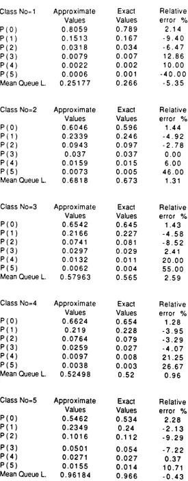
The algorithm is applied to a variety of multi-class queues with different number of classes, window capacities, arrival rates and service rates. A representative set of examples were given in Tables 2-8. Exact values for the validation purposes are obtained numerically for the three class model and using a simulation program (written in QNAP) for four and five classes. Relative error percentages are calculated as 100*(exact value-approximate value)/exact value.

3. Network of Queues

In this section, we discuss the applicability of the algorithm developed in section 2 to network of queues in which each queue is a multi-class queue with class dependent window-flow control as studied above.

(14)

There are N classes of jobs arriving at queue 1 in

a

poisson fashion with a class dependent rate Ak' Each class k has its own window size at queue i, wik' i=1, ... ,K; k=1, ... ,N, where K is the number of queues in the network. Each queue in the network is of the type considered in this paper, as illustrated in Figure 1.

A

job, completing its service at queue i, joins queue j with probability Pij, which is independent of the class of the job. The state of this network is a vector of vectors

(S, ,...

,8_{K ) ,} where Si=(Si1 ,...,SiN)· Sik denotes the number of class k jobs at queue i. As each queue in isolation do not have a product form solution, we should expect that the network of queues do not have a product form solution as well.

Let us now consider the network after aggregating all classes into a single class. The arrival rate of this single class is the sum of the arrival

N

rates of all classes, Le.AA= L)-'k' The state of the network is (n1,· .. ,nK),

k=1

where ni is the total number of jobs (all classes) at node i. In this case, from theorem 1, the network reduces to K independent M/M/1 queues. Let P(.) be the joint steady state queue length distribution of the total number of jobs at each queue and Pi(ni) be the marginal probability of having nj jobs at queue i, which can be obtained by analyzing the queue in isolation. Then:

P(n1 ,...,nK)=P1(n, )P_{2(n2)····PK(nK)}

N

where P_j(nj)=(1-p)pni, p= LAi/Jli' Hence, the performance measures of the i=1

(15)

classes. In particular, the departure process of each class is not exponential, hence, the arrival distribution of class k jobs at queue i, i/:1, is not poisson. Considering the fact that the state space of this network is very large, it may not be possible to solve it numerically, and simulating the network is expected to be very time consuming.

As an approximate solution technique, we decompose the network into individual queues and analyze them in isolation.

By

doing so, only the arrival processes need to be characterized, as the other parameters of the queue in isolation, Le. window-sizes, service rate, should be the same as in the original network. Let us first assume that arrival of class k jobs to each queue occurs in a poisson fashion. The total arrival stream of class k jobs into queue i is formed by class k departures from other queues that are routed to queue L Hence, the arrival rate of class k jobs into queue i, Yik' is the solution of the traffic equations:

K

'Yik=A.j+ L'YjkPji, i=1, ... ,K j=1

(16)

We presented a model for the case where multiple connections use the same resource, depicted by a single server queue. As the numerical approach becomes infeasible even with a few classes, it is necessary to develop approximation algorithms for the analysis of such queues. An approximation algorithm is developed based on decomposing the queue into N-class queues where N is the number of classes. These two-class models are then solved numerically using Neuts' matrix geometric procedure. Validation tests show that the algorithm is very accurate. The applicability of the algorithm to the network of queues is immediate after decomposing the network by node. In this case, the only assumption required is poisson arrivals to each queue.

(17)

REFERENCES

[1] S. Fdida, H.G. Perras, and A. Wilks, "Semaphore Queues: Modelling multilayered Window Flow Control Mechanisms", Tech. Rep. Computer Science, 1988, North Carolina State University

[2] A. Krzeinski and P. Teunissen, "Multiclass Queueing Networks with Population Constrained Subnetworks", Proc. ACM Sigmetrics Cant. on Measurement and Modelling Computer Systems, Austin, TX, 1985, 128-139

[3] S.S. Lam, "Queueing Networks with Population Size Constraints", IBM

J.

Res. Dev., July 1977, 370-388

[4] E.D. Lazowska and J. Zahorjan, "Multiple Class Memory Constrained Queueing Networks", Proc. ACM SIGMETRICS Cont. on Measurement and Modeling of Computer Systems, Seattle WA, 1982, 130-140

[5] M.F. Neuts, Matrix Geometric Solutions in Stochastic Models-An algorithmic approach, The John Hopkins University Press, Baltimore, 1981

[6] R. Onvural, H.G. Perros, and U. Koerner, "On a Multi-Class Queue with Class Dependent Window-Flow Control", 4th Int. Cont. on Modelling Tech. and Tools for Compo Perf. Evaluation

[7] M. Reiser, "A Queueing Network Analysis of Computer Communications Network with Window Flow Control", IEEE Trans. Comm., vel. COM 27, 1199-1209, 1979

[8] M. Reiser, "Performance Evaluation ot Data Communications Systems", Proc. IEEE, vol. 70, 1982, 171-196

(18)

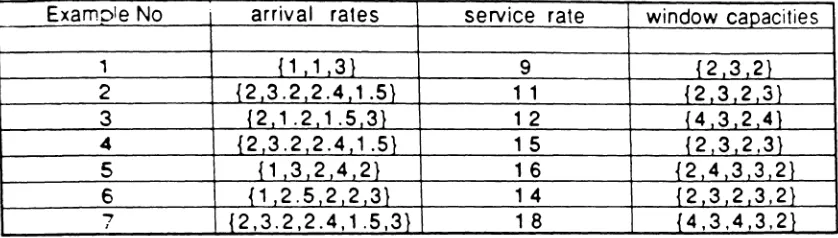
Table 1: Data for the examples in tables 2 to 8

ExamDleNo arrival rates service rate window capacities

,

{1 1 31 9 {2 3 2}

2 {2.3.2 2.4 1 .51 11 {2,3 2,31

3 f2.1.2 1.5 3) 1 2 {4,3.2,41

4 {2 3.2 2.4 1 .5) 1 5 {2 3,2,3)

5 {1 3 2,4 2) 1 6 {243321

6 {1 2.5 2,2,31 1 4 {2 3 2 3,2)

7 {2,3.2,2.4,1.5,3) 1 8 {4,3,4,3,2}

Table 2: Example 1 in Table 1

Class No=1 Approximate Exact Relative Values Values error 0/0

P(O) 0.8118 0.8082 0.45

P ( 1 ) 0.1493 0.156 -4.29

P(2) 0.0299 0.0284 5.28

P(3) 0.0068 0.0057 19.30

P(4} 0.0016 0.0012 33.33

P(5) 0.0004 0.0003 33.33

Mean Queue L. 0.2387 0.2367 0.84

Class No=2 Approximate Exact Relative Values Values error %

P(O) 0.8113 0.809 0.28

P ( 1 ) 0.1499 0.1563 -4.09

P(2) 0.0308 0.0286 7.69

P(3) 0.0063 0.0051 23.53

P(4) 0.0014 0.0009 55.56

P(5) 0.0003 0.0002 50.00

Mean Queue L 0.23755 0.23315 1.89

ClassNo=3 Approximate Exact Relative Values Values error %

P(O) 0.5744 0.5705 0.68

P ( 1 ) 0.2402 0.2427 -1 .03

P(2) 0.1 009 0.1018 -0.88

P(3) 0.0446 0.0449 -0.67

P(4) 0.0206 0.0207 -0.48

P(5) 0.0098 0.0098 0.00

(19)

Table

3:

Example 2 in Table 1

Class No=' Approximate Exact Relative Values Values error %

P(O) 0.4921 0.478 2.95

P ( , ) 0.2566 0.25 2.64

P(2) 0.11 54 0.128 - 9.84

P(3) 0.0591 0.064 -7.66

P(4) 0.0324 0.036 -10 .00

P(5) 0.0185 0.019 -2.63

Mean Queue L. 1.078 1.085 -0.65

P(O) 0.3801 0.37 2.73

P ( 1 ) 0.2459 0.238 3.32

P(2) 0.1453 0.148 -1 .82

P(3) 0.0827 0.091 - 9.1 2

P(4) 0.0505 0.057 -11.40

P(5) 0.0321 0.036 -10.83

Mean QueueL. 1 .654 1.7009 -2.76

P(O) 0.4427 0.407 8.77

P ( , ) _0.2486 _0.232 _7.16

P(2) 0.1231 0.134 - 8.1 3

P(3) 0.0691 0.076 -9.08

P(4) 0.0417 0.047 -.11.28

P(5) 0.0262 0.031 -15.48

Mean QueueL. 1.3824 1 .4334 -3.56

P(O) 0.578 0.583 -0.86

P ( 1 ) 0.2645 0.261 1.34

P(2) 0.1003 0.101 -0.69

P(3) 0.0359 0.037 -2.97

P(4) 0.0133 0.012 10.83

P(S) 0.0049 0.004 22.50

(20)

Table

4:

Example

3

in Table 1

ClassNo=1 Approximate Exact Relative

Values Values error 0/0

P(O) _0.6864 _0.685 _0.20

P ( 1 ) 0.2145 0.216 .. 0.69

P(2) 0.0677 0.069 -1 .88

P(3) 0.0213 0.021 1.43

P(4) _0.0066 _0.007 _-5.71

P(5) 0.0022 0.002 10.00

Mean Queue L. 0.4592 0.455 0.92

P(O) 0.7863 0.784 0.29

P ( 1 ) 0.1672 0.17 -1 .65

P(2) 0.0362 0.036 0.56

P(3) 0.0078 0.008 -2.50

P(4) 0.0019 0.0017 11 .76

P(5) 0.0005 0.0003 66.67

Mean Queue L. 0.27384 0.2743 - 0.1 7

P(O) 0.7437 0.735 1 .1 8

P ( 1 ) 0.1876 0.192 -2.29

P (2) 0.0473 0.053 .. 10.75

P(3) 0.0139 0.015 -7.33

P(4) 0.0046 0.004 1.5.00

P(5) 0.0017 0.001 70.00

Mean Queue L. 0.35763 0.364 -1 .75

Class No=4 Approximate Exact Relative

P (0) 0.5913 0.589 0.39

P ( 1 ) 0.2407 0.242 -0.54

P(2) 0.0986 0.099 -0.40

P(3) 0.0402 0.041 -1 .95

P(4) 0.0162 0.018 -10.00

P(5) 0.0069 0.007 -1 .43

(21)

Table 5: Example 4 in Table 1

P(O) 0.7522 0.746 0.83

P ( 1 ) 0.1832 0.187 -2.03

P(2) 0.0454 0.049 -7.35

P(3) 0.0129 0.013 -0.77

P(4) 0.0041 0.004 2.50

P(5) 0.0014 0.00 1 40.00

Mean Queue L. 0.34074 0.345 -1 .23

P(O) 0.653 0.652 0.15

P ( 1 ) 0.2247 0.226 - 0.58

P(2) 0.0783 0.078 0.38

P(3) 0.027 0.027 0.00

P(4) 0.0101 0.01 1.00

P(5) 0.004 0.004 0.00

Mean QueueL 0.5421 0.538 0.76

P(O) 0.7151 0.711 0.58

P ( 1 ) 0.2 0.202 -0.99

P(2) 0.0564 0.06 -6.00

P(3) 0.0181 0.018 0.56

P(4) 0.0064 0.006 6.67

P(5) 0.0024 0.002 20.00

Mean Queue L. 0.41499 0.416 -0.24

Class No=4 Approximate Exact Relative

Values Values error %

P(O) 0.8052 0.801 0.52

P ( 1 ) 0.1554 0.16 -2.88

P(2) 0.0314 0.031 1.29

P(3) 0.0063 0.006 5.00

P(4) 0.0014 0.001 40.00

P(5) 0.0003 0.001 _-70.00

(22)

Class No=1

P{O)

P ( 1 )

P(2) P(3) P(4) P(5)

Mean Queue L.

ClassNo=2

P{O) P (1 )

P(2) P(3) P(4) P(5)

Mean Queue L

Class No=3

P(O)

P ( 1 )

P(2) P(3) P(4) P(5)

Mean Queue L.

ClassNo=4

P(O) P ( 1 ) P(2) P(3) P(4)

P(S)

Mean Queue L.

Class No=S

P(O)

P (1 )

P(2) P(3) P(4) P(5)

Mean Queue L.

(23)

P(O) 0.8059 0.789 2.14

P (1 ) 0.1513 0.167 - 9.40

P(2) 0.0318 0.034 - 6.47

P(3) 0.0079 0.007 12.86

P(4) 0.0022 0.002 10.00

P(S) 0.0006 0.001 -40.00

Mean Queue L. 0.25177 0.266 -5.35

P(O) 0.6046 0.596 1.44

P ( 1 ) 0.2339 0.246 -4.92

P(2) 0.0943 0.097 - 2.78

P(3) 0.037 0.037 0.00

P(4) 0.0159 0.015 6.00

P(5} 0.0073 0.005 46.00

Mean Queue L. 0.6818 0.673 1 .31

P(O) 0.6542 0.645 1.43

P ( 1 ) 0.2166 0.227 -4.58

P(2) 0.0741 0.081 -8.52

P(3) 0.0297 0.029 2.41

P(4) 0.0132 0.011 20.00

P(S) 0.0062 0.004 55.00

Mean Queue L. 0.57963 0.565 2.59

P(O) 0.6624 0.654 1.28

P ( 1 ) 0.219 0.228 -3.95

P(2) 0.0764 0.079 -3.29

P(3) 0.0259 0.027 -4.07

P(4) 0.0097 0.008 21.25

P(5) 0.0038 0.003 26.67

Mean Queue L. 0.52498 0.52 0.96

P(O) 0.5462 0.534 2.28

P ( 1 ) 0.2349 0.24 - 2.13

P(2) 0.1016 0.112 -9.29

P(3) 0.0501 0.054 -7.22

P(4) 0.0271 0.027 0.37

P(5) 0.0155 _0.014 _10.71

(24)

22

Class No=1 _Approximate _Exact _Relative Values Values error %

P(O) 0.7554 0.751 0.59

P ( 1 ) _0.183 _0.188 _{- 2.66}

P(2) 0.046 0.046 0.00

P(3) 0.0115 0.011 4.55

P(4) _0.0029 _0.003 _-3.33

P(5) 0.0008 0.001 -20.00

Mean Queue L. 0.32706 0.329 -0.59

P(O) 0.6538 0.648 0.90

P ( 1 ) 0.2235 0.228 -1 .97

P(2) 0.0779 0.08 - 2.63

P(3) 0.0267 0.03 -11.00

P(4) 0.01 02 0.009 13.33

P(5) 0.0042 0.003 40.00

Mean Queue L. 0.54597 0.542 0.73

P(O) 0.7187 0.714 0.66

P ( 1 ) 0.2003 0.207 -3.24

P(2) 0.0577 0.058 - 0.52

P(3) 0.0165 0.016 3.13

P(4) 0.0047 0.005 - 6.00

P(5) 0.0014 0.001 40.00

Mean Queue L. 0.39535 0.396 - 0.1 6

P(O) 0.8064 0.801 0.67

P ( 1 ) 0.1544 0.16 -3.50

P(2) 0.0311 0.031 0.32

P(3} 0.0062 0.007 -11.43

P(4) 0.0014 0.001 40.00

P(S) 0.0004 0.001 -60.00

Mean Queue L. 0.24328 0.247 -1 .51

Class No=S Approximate Exact Relative Values Values error %

P(O) 0.6661 0.658 1.23

P ( 1 ) 0.2162 0.222 -2.61

P(2) 0.0-704 0.075 - 6.13

P(3) 0.0264 0.028 -5.71

P(4) 0.0111 0.01 11 .00

P(5) 0.005 0.004 25.00