Full and Model Reduced Structure Preserving Simulation of Incompressible Fluids

Incompressible Fluids

Thesis by

Gemma Mason

In Partial Fulfillment of the Requirements for the Degree of

Doctor of Philosophy

California Institute of Technology Pasadena, California

2015

c

2015

Acknowledgements

Every long road has a long list of people who helped along the way. Let me start by thanking my adviser, Mathieu Desbrun, for a great deal of advice and help, and for being such an important part of allowing me to fit in here at Caltech.

I owe a deep debt of gratitude to Christian Lessig, who provided me with support and mentor-ship, without which this PhD would not have been worth as nearly as much to me.

Particular thanks to Beibei Liu and Yiying Tong for their significant contributions to the results presented in Chapter 4. Thanks are also due to Dmitry Pavlov, Patrick Mullen and Dzhelil Rufat for valuable discussions and collaborations, and to Tudor Ratiu and Fran¸cois Gay-Balmaz, who gave advice both via email and in person.

The late Jerry Marsden was my co-adviser for a very brief time. His advice for that short time was shrewd and nurturing. I am sorry not to have been able to know him longer.

Finally, let me thank my family and my fianc´e. Mum, your sympathy has been a great comfort to me. Dad, your unfailing belief in me has helped to steer me through times of trouble. Hannah, Kathryn, and Annie, I love you all and you make my life so much brighter. Paddy, I don’t know how I’d have done this without you.

Abstract

This thesis outlines the construction of several types of structured integrators for incompressible fluids. We first present a vorticity integrator, which is the Hamiltonian counterpart of the exist-ing Lagrangian-based fluid integrator [32]. We next present a model-reduced variational Eulerian integrator for incompressible fluids, which combines the efficiency gains of dimension reduction, the qualitative robustness to coarse spatial and temporal resolutions of geometric integrators, and the simplicity of homogenized boundary conditions on regular grids to deal with arbitrarily-shaped domains with sub-grid accuracy.

Both these numerical methods involve approximating the Lie group of volume-preserving diffeo-morphisms by a finite-dimensional Lie-group and then restricting the resulting variational principle by means of a non-holonomic constraint. Advantages and limitations of this discretization method will be outlined. It will be seen that these derivation techniques are unable to yield symplectic integrators, but that energy conservation is easily obtained, as is a discretized version of Kelvin’s circulation theorem.

Contents

Acknowledgements iv

Abstract v

1 Introduction 1

1.1 Contributions . . . 3

2 Summary of Lagrangian Fluids 4 2.1 Continuous theory . . . 4

2.2 Discretization process . . . 6

2.2.1 The finite-dimensional Lie group method . . . 6

2.2.2 Discrete exterior calculus . . . 7

2.2.3 Non-holonomic constraint . . . 9

2.2.4 Discrete flat operator and inner product . . . 9

2.3 Creating a variational numerical method . . . 10

2.4 Results and Discussion . . . 11

3 Hamiltonian Fluids 13 3.1 Review of continuous theory . . . 14

3.2 Derivation . . . 15

3.2.1 Preliminary theoretical elements . . . 15

3.2.2 Variational derivation . . . 17

3.2.3 Derivation from a discrete version of the Lie-Poisson bracket . . . 19

3.2.5 Time discretization . . . 21

3.2.6 Explicit numerical formulas . . . 23

3.3 Results . . . 25

3.4 Discussion . . . 29

4 Model-Reduced Lagrangian Fluids 30 4.1 Derivation . . . 31

4.1.1 Spectral Bases . . . 31

4.1.2 Non-holonomic constraint. . . 33

4.1.3 Implementation . . . 35

4.1.4 Spectral variational integrator . . . 38

4.1.5 Kelvin’s circulation theorem . . . 40

4.2 Results . . . 41

4.2.1 Generalization to other bases . . . 44

4.3 Discussion . . . 48

4.3.1 Persistence of non-holonomic constraints . . . 48

5 Spectral Discrete Exterior Calculus 50 5.1 Basic Spectral Tools . . . 51

5.1.1 Reduction and Reconstruction Maps . . . 51

5.1.2 1D Periodic Interpolator & Histopolator Functions . . . 53

5.1.3 Spectral Basis Functions on Regular Grids . . . 54

5.1.4 Chebyshev Grids over Bounded Domains . . . 56

5.2 Spectrally Accurate Discrete Operators . . . 62

5.2.1 Discrete Exterior DerivativeD . . . 62

5.2.2 Discrete Wedge ProductW . . . 63

5.2.3 Discrete Hodge StarH. . . 64

5.3 Discussion . . . 66

6 Conclusion 68

Chapter 1

Introduction

Imitating continuous structures in order to produce numerical integrators that preserve geometric properties of the problem being approximated is a technique that has been used in a wide variety of contexts in recent decades. Within the field of ordinary differential equations, the study of geometric integrators is very well developed [17]. In particular, the technique of variational integration [43], which imitates the action integral via a sum over discrete times, was developed in order to reliably create symplectic integrators for ODE systems.

Structured integrators for partial differential equations are a more recent and less well-developed subject, but considerable strides have been made in recent years in subjects such as electromagnetics [38] and Lagrangian field theories [41]. 2011 saw the publication of a structure-preserving integra-tor for incompressible fluids [32], which discretized Arnold’s classic formulation of incompressible, inviscid fluids in terms of geodesics on the Lie group of volume-preserving diffeomorphisms. This paper drew on earlier techniques such as discrete exterior calculus [11] and the discrete action [43], but it also introduced the completely new technique of approximating the infinite-dimensional Lie group of volume-preserving diffeomorphisms by a finite-dimensional Lie group. Techniques such as discrete exterior calculus and the finite-dimensional Lie group method are structure-preserving discretizations in space, and may be employed either separately or together with existing variational integrators in time.

be achieved either variationally or by means of a discrete Lie-Poisson bracket. We also derive discrete Lie-Poisson integration in time. These developments may be viewed as analogous to the development of discrete Hamiltonian variational integrators for ordinary differential equations [43]. A notable disadvantage of these earliest geometric fluids methods [32], [14] is the large num-ber of variables involved. These arise as a result of the discretization of the space into a large number of cells, all of which may theoretically interact with one another. In practice, we are able to restrict interactions to nearest neighbors by means of a non-holonomic constraint. However, further reduction in the number of variables and in the computational time would be desirable, particularly for applications in fluid animation. For this reason, we turn to the techniques ofmodel reduction, approximating the fluid motion using only a small number of basis functions in the style

of computational fluid dynamics methods such as [35, 45, 31]. Dimensionality reduction was first introduced for fluid animation by Treuille et al. [40] through Galerkin projection onto a reduced set of basis functions computed through principal component analysis of a training set of fluid motion. A number of works followed proposing the use of different bases such as Legendre polyno-mials [16], trigonometric functions [24], or even non-polynomial Galerkin projection [37]; eventually, Laplacian eigenvectors were pointed out by [10] to be particularly appropriate, as they guarantee divergence free flows and facilitate the conversion between vorticity and velocity, while offering a sparse advection operator for regular domains. These eigenfunctions also allow easy implementation of viscosity.

Chapter 4 presents a model-reduced variational integrator. Interestingly, despite the smaller space of variables, this method still requires a non-holonomic constraint, which will prompt some important theoretical insights. We use spectral approximation of the functional map through (cell-based) scalar and (face-(cell-based) vector Laplacian eigenvectors in order to offer model reduction without losing the variational properties of the integrator. Furthermore, we extend the embedded-boundary approach of [30] to our framework in order to compute spectral (scalar- and vector-valued) basis functions of arbitrary domains directly on regular grids for fast computations with sub-grid accuracy We demonstrate the efficiency of our resulting integrator through a number of examples in 2D, 3D, and curved 2D domains.

of a spectral discrete exterior calculus, which may be of use in creating a structured fluid integrator which does not employ a finite-dimensional Lie group.

Together, these new developments in the structure-preserving simulation of incompressible fluids significantly increase our theoretical understanding of the application of variational and geometric methods to the mathematics of fluid motion.

1.1

Contributions

• Chapter 2 reviews the work of Pavlov et al [32], emphasising the techniques used and outlining

some of its limitations.

• Chapter 3 presents a new Hamiltonian integrator for incompressible fluids (work done with

the mentorship of Christian Lessig).

• Chapter 4 presents a model-reduced integrator, using Laplacian eigenfunctions to improve

the computation speed (work done in collaboration with Beibei Liu, Yiying Tong, and my adviser).

Chapter 2

Summary of Lagrangian Fluids

This chapter will outline structure-preserving integrators for inviscid, incompressible fluids as de-veloped in [32] and [14]. We will see how to mimic the Lie group Lagrangian structure of the fluid (as discovered by Arnold in 1966 [2]) in a discretized form. This allows us to create integrators with good energy behavior, and that preserve a discrete version of Kelvin’s circulation theorem. We will see in later chapters that elements of the process used here may be applied to a wide variety of structure-preserving integrators for fluids.

2.1

Continuous theory

The variational understanding of incompressible fluids is based upon the observation by Arnold [2] that the motion of an incompressible, inviscid fluid on a manifoldM(possibly with boundary) may be derived as geodesic motion on the infinite-dimensional Lie group Diffvol(M) of

volume-preserving diffeomorphisms on that manifold. Specifically, the position of the fluid at time t is represented by a diffeomorphismφt, which represents the change in position of each fluid particle

when we change from time 0 to time t. Because the fluid is incompressible, this diffeomorphism will be volume-preserving.

This Lie group representation is Lagrangian in that it records the motions of specific particles1_.

The associated Eulerian representation, which records the velocity field at each fixed point in space, may be obtained by moving to the associated Lie algebraχdiv, consisting of the divergence-free

vector fields on the manifoldMwhich are parallel to the boundary, ifMhas a boundary. We can find the appropriate geodesic motion by solving for the time-dependent velocity fieldv(x, t), which is a stationary point of the actionRt

0Ldt, where the Lagrangian functionLis defined by

L=

Z

M

kvk2_{dV, (2.1)}

wherekvk uses the standard Euclidean norm on vectors inRn, and the variations satisfy the Lin

constraints:

δv= ˙ξ+ [v, ξ]. (2.2)

A Lagrangian stationary action problem of this type, which uses Eulerian rather than Lagrangian co-ordinates, is solved by the Euler-Poincar´e equations [9], which are similar to the Euler-Lagrange equations for Lagrangian co-ordinates. In this case, the resulting equations are

˙

v[+Lv(v[) =−dp, (2.3)

wherev[ _{is the 1-form dual to the vector fieldv,L}

v is the Lie derivative with respect tov, and dp

is the exterior derivative of some 0-formp.

On regions inR2 or R3, these equations are equivalent to the expected Euler equations for an

incompressible, inviscid fluid:

∂v

∂t +v· ∇v=−∇P, (2.4)

whereP is a function which accounts for the pressure.

Arnold’s Lagrangian derivation can be used to show that Kelvin’s theorem holds. Specifically, the circulation-preservation required by Kelvin’s theorem is a special case of Noether’s theorem, which states that a continuous symmetry of a Lagrangian system induces a conserved momentum. In this case, the Lagrangian is conserved under a particle-relabeling symmetry. That is, if we relabel each fluid particle by rearranging them according to some volume-preserving diffeomorphism

2.2

Discretization process

The 2011 paper of Pavlov et al [32] introduced a variational integrator for fluids, based on the continuous variational derivation of Euler fluids as geodesics on χvol. This method used several

varieties of geometric discretization at once. Most notably, it introduced the idea of approximation of the infinite dimensional Lie group of volume-preserving diffeomorphisms with an appropriate finite-dimensional Lie groupG. It also introduced a new variant on discrete exterior calculus [11] which interacts with the associated Lie algebrag. With the help of a non-holonomic constraint, these two elements can spatially discretize the motion of the fluid in a manner that respects the Lagrangian structure. It is then possible to derive an associated time-discretization using the method of a discrete variational principle, a geometric discretization method that has been extensively developed

for use with ODEs [43].

I shall detail here the main elements of the spatial discretization.

2.2.1

The finite-dimensional Lie group method

To find a finite-dimensional Lie group that can approximate the behavior of the infinite-dimensional Lie group Diffvol(M), we begin by discretizing the fluid domain into a finite number of cells. In

preparation for the rest of this thesis, the explanation given here will focus on regular Cartesian grids, with square cells of widthh.

We discretize a continuous functionf(x) on the manifoldMby taking an average (integrated) value fi per grid cell i of the mesh, which we arrange in a vector f. This definition of discrete

functions allows us to discretize the set of possible flowsφt∈Diffvol(M) using a Koopman operator

(orfunctional map, as it is known in computer graphics literature), which describes the action of the flow in terms of how it changes a discrete function. Specifically, the flow map is encoded as a matrixqof size the square of the number of cells, and the integrated values f off per cell become

qf oncef is advected by the flowφ.

The constant function is unchanged when advected by the flow, so every discrete flow should take the constant function to itself. That is, for allq, we require thatq1=1,where1is a vector of ones (see [32] for the equivalent condition on an arbitrary mesh). This is the same as saying that the row sums ofqare equal to 1, i.e.,q issigned stochastic.

volume-preserving. This condition is achieved by asking that the discrete flow preserves the inner product of vectors, that is, q isorthogonal, i.e., qT_=q−1_{. Thus, we find that we need to takeq to be an}

element of the Lie groupGof orthogonal, signed stochastic matrices. This matrix group represents our discrete fluid configuration, as we describe next.

We can view the finite-dimensional Lie groupGas a configuration space: it encodes the space of possible “positions” for the discrete fluid, in that each element of the Lie group represents a possible way that the fluid could have evolved from its initial position. This Lie group represents a Lagrangian perspective as it identifies the fluid particles in a given cell by recording which cells they originally came from. The associated Eulerian perspective is given by the Lie algebragof matrices of the form ˙q◦q−1 _{forq∈G. It was shown in [32] that any matrixA∈gof this Lie algebra is both}

antisymmetric (AT_{=−A) androw-null (A1=0), and corresponds to a discrete counterpart of the}

Lie derivativeLv with respect to the continuous velocity fieldv= ˙φ◦φ−1. Thus, the product Af

of such a matrix with a discrete functionf approximates the continuous termv· ∇f. Furthermore, if cellsi andj are nearest neighbors, then the matrix elementAij represents the flux of the fluid

through the face shared by cellsiandj. Thus, an element of the Lie algebragofGis directly linked to the usual flux-based (Marker And Cell) discretization of vector field in fluid simulators [18].

2.2.2

Discrete exterior calculus

The Lie algebrag consists of vector fields on our discrete manifold. The space Ω1 of functionals

on these vector fields may therefore be viewed as a space of discrete 1-forms, while the integrated functions f that we defined above would naturally form the space Ω0 of discrete 0-forms. This

suggests that we might be able to form some sort of discrete exterior calculus [11], defining discrete versions of operators such as the exterior derivative, which will be of use in describing the motion of a discrete fluid.

Throughout this thesis, the discrete versions of continuous operators will be indicated by bold-face. For example, the continuous exterior derivative is written as d, and the discrete exterior derivative (defined below) will be denotedd.

We define the space of discrete 1-forms Ω1 as the space of antisymmetric matrices. We pair a 1-formC[ _{with a vector fieldB using a Frobenius pairing:}

2-forms are defined in this formulation as antisymmetric 3-tensorsFijk. We define thecontraction

of a 2-formF with a vector fieldA as

(iAF)ij =

X

k

(FikjAik−FjkiAjk) , (2.6)

which is constructed to be antisymmetric so as to yield a 1-form. It was shown in [32] that this definition is consistent with defining the total pairing of a 2-formF with two vector fields A,B as

hF, A, Bi=X

i,j,k

FijkAijBik. (2.7)

We can now define a discrete exterior derivative which takes us from a vectorfof function values (f1, f2, ...fN) to an antisymmetric matrix as follows:

Aij = (df)ij =fi−fj. (2.8)

The exterior derivative on 1-forms is similarly defined by antisymmetry as:

(dA)ijk=Aij+Ajk+Aki. (2.9)

More generally, a k-form is given by an antisymmetric (k+1)-tensor, and the discrete exterior derivative on ak-form is

dGi1i2···ik+1=

X

j∈{1,2,···,k+1}

(−1)j+1Gi1···ij−1ij+1···ik+1. (2.10)

The discrete exterior derivative satisfies d2 _{= 0, as we would expect by comparison with the}

continuous version of the operator.

the construction of the discrete flat operator in Section 2.2.4.

2.2.3

Non-holonomic constraint

Whilst the elements Aij for A∈g have a clear physical interpretation in the case where i and

j are nearest neighbors, this is not the case for elements representing interactions between cells that are not immediate neighbors. Similarly to a CFL condition, we prohibit fluid particles from skipping to non-neighboring cells by restricting the Lie algebra to the constrained set S, the set of matrices A such that Aij= 0 unless cells i and j share a face (or an edge in 2D). We require

the elements of g that we use to represent the fluid velocity fields to fall into this constrained set. This has the additional advantage of making the matrices sparse, dramatically decreasing the amount of memory required and the computational time, as much fewer degrees of freedom need to be updated. Moreover, a Lie algebra element in this constrained set corresponds exactly to the traditional MAC discretization with fluxes. We can also relate fluxes between nearest neighbors to the fluxes on edges that are used in discrete exterior calculus [11].

Constraining the matrices in this way requires a non-holonomic constraint, because the set S

is not closed under the Lie bracket. That is, interactions between nearest neighbors followed by further interactions between nearest neighbors produce interactions between cells that are two-away from each other, which are therefore not inside the constrained setS.

2.2.4

Discrete flat operator and inner product

The co-ordinate-independent nature of exterior calculus allows us to translate it to the discrete setting with the structure intact, in such a way that no error whatsoever is introduced by the discretization process. However, all numerical methods introduce error at some point, and with numerical methods derived from discrete exterior calculus that error comes from places in the method where the co-ordinates (and thus the local metric) must unavoidably be introduced. The method of Pavlov et al [32] does this by introducing both an inner product and a flat operator, which takes a vector fieldA∈gand maps it to the 1-formA[∈g∗ such that

where the angle brackets on the left hand side indicate the pairing of a 1-form with a vector field (2.5), and the curved brackets on the right hand side indicate an inner product between vector fields. We use a Frobenius inner product between vector fields as follows:

(A, B) = 2h2Tr(ATB) (2.12)

wherehis the spatial step size. This definition approximates an integral of the product of the two functions over the spaceM.

One might think that condition (2.11) would be sufficient to define the flat operator. This turns out not to be the case. Equation (2.11) only defines those elements ofA[ _{that record interactions}

between cells that are nearest neighbors. However, we will also need to know the entries ofA[_for

pairs of cells that share a nearest neighbor in common. To define these elements ofA[_{, we require}

that the flat operator satisfies the following condition on the total pairing of its discrete exterior derivative with two discrete vector fields:

hdA[, B, Ci →

Z

M

dv[(u, w)dV (2.13)

ash→0, whereA, B andC converge tov,uandw, respectively, as h→0. It was shown in [32] that this may be achieved with a little help from discrete exterior calculus to determine the desired form of the vorticity elementsdA[_{. I refer the reader to this paper for more details.}

2.3

Creating a variational numerical method

Using the spatial discretization outlined in the preceding section, Pavlov et al [32] showed that one can create a semidiscretized numerical method for ideal, incompressible fluids through the Euler-Poincar´e equations [14] for the Lagrangian given by

Lsemidiscrete=

1

2(A, A)≈ 1 2

Z

where variations of A satisfy the Lin constraint δA = ˙B+ [A, B], and A is subject to the non-holonomic constraintA∈ S. This gives the equations

˙

A[+LAA[=−dp. (2.15)

Because the semidiscretized equations constitute a Lagrangian system of ODEs, they may be discretized in time using the method of a discrete Lagrangian [43]. The resulting equations are equivalent to the Harlow-Welch Scheme [18] with a Crank-Nicolson (trapezoidal) update rule. Al-ternatively, we may create an energy-preserving method by updating with the midpoint rule [28].

2.4

Results and Discussion

We see that the technique of representing the Lie group structure of Diffvol(M) using an appropriate

finite dimensional Lie group may be used, together with a version of discrete exterior calculus and a non-holonomic constraint, in order to construct a numerical method for fluids which discretizes in space in a way that preserves the variational structure. Time discretization may then be achieved either by the energy-preserving midpoint rule, or using a discrete-time variational integrator.

Chapter 3

Hamiltonian Fluids

Arnold’s geodesic formulation of inviscid, incompressible fluids has an associated Hamiltonian for-mulation, as described by Marsden and Weinstein [26]. The primary variable in the Hamiltonian viewpoint is thevorticity rather than the velocity. This chapter describes a numerical method for fluids based on this Hamiltonian vorticity viewpoint.

Expanding our understanding of geometric numerical methods for fluids to the Hamiltonian perspective is useful from a practical perspective, in that the stream function is located on points, a property which may be useful for constructing embedded boundary methods. Specifically, if there is no fluid flow through the boundary, then the stream function is constant on the boundary. If the boundary is connected, then without loss of generality we may set the stream function to zero there. If we then wish to consider the flux through an edge that passes through an embedded boundary, we may find it by subtracting the boundary value of the stream function from the value of the stream function at one of the edge’s two vertices, taking the vertex located inside the boundary.

Although the vorticity form of the Euler equations is generally used in two dimensions, the framework of differential forms does allow it to be used in three dimensions as well [26]. However, in this thesis we will consider only the two-dimensional case.

3.1

Review of continuous theory

Recall from Section 2.1 that the motion of an incompressible fluid may be described by elements of Diffvol(M), the Lie algebra of volume-preserving diffeomorphisms, or in the Eulerian sense by

elements of χdiv, the Lie algebra of divergence-free vector fields. The Lagrangian L is invariant

under a particle-relabeling symmetry: for any g ∈ Diffvol(M), L(gR(v)) = L(v) for v ∈ χdiv,

where gR(v) is the right action ofg onv. Marsden and Weinstein showed in 1983 [26] that this

symmetry allows us to perform a Lie-Poisson reduction in order to induce a Hamiltonian system on the dual space χ∗_div. This dual space consists of 1-forms modulo exact 1-forms (in the Euler equations for an incompressible fluid, the modulo over exact 1-forms is accounted for by the dp

term). Equivalently, we may identify any element ofχ∗_divwith an exact 2-form via a bijection given by the exterior derivative1_{. Taking the exterior derivative of a 1-form is equivalent to taking the}

curl of the associated vector field, and this bijection takes us from a given velocity to the associated vorticity.

Since we have only kinetic (and not potential) energy, when we move to the Hamiltonian picture the Hamiltonian function is equal to our earlier Lagrangian (2.14), transformed into momentum co-ordinates. Given homogeneous boundary conditions (so that the codifferentialδwill be the adjoint of the exterior derivative), this transformation is as follows:

H = (v[, v[) (3.1a)

= (δd∆−1v[, v[) (3.1b)

= (∆−1dv[,dv[) (3.1c)

= (∆−1ω, ω). (3.1d)

Note that the Laplace-deRham operator ∆v[_{= (δd + dδ)v}[_=δdv[ _{since the codifferentialδv}[_{= 0}

becausevis divergence-free. A similar formula holds forω, where we have ∆ω= (δd + dδ)ω= dδω, because dω= 0. I have also used the fact that d commutes with ∆−1_{. This follows easily from the}

fact that d commutes with ∆, which can be verified using the definition of ∆ and the nilpotence of the exterior derivative.

(derived via momentum reduction):

where δF_δω ∈χdiv is a functional derivative and an element of the Lie algebra. Then the Lie-Poisson

equations ˙F={F, H}yield the vorticity equations:

∂ω

∂t +Lvω= 0 (3.3a)

with ω= dv. (3.3b)

More recently, Cendra et al [9] explained how to derive the Lie-Poisson equations from a varia-tional principle. In the context of incompressible fluids, the Lie-Poisson variavaria-tional principle states that the curve (v(t), ω(t))∈χdiv×χ∗div is a critical point of the action

This variational principle is equivalent both to Hamilton’s principle of critical action and to the Lie-Poisson equations, which are equivalent to the vorticity equation (3.3a) given above.

3.2

Derivation

3.2.1

Preliminary theoretical elements

By analogy with the continuous theory, we convert a velocity into a vorticity by moving from the space Ω1/dΩ0 of discrete 1-forms modulo exact discrete 1-forms to the space Ωex2 of exact discrete

2-forms. A bijectionβ(A) =dA[_{between the two spaces is given by the discrete exterior derivative.}

Thus, we define the vorticity 2-formW =dA[_{to be the discrete exterior derivative of the velocity}

1-form.

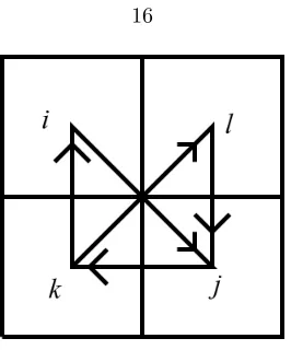
Figure 3.1: The square cellsi, j,k andl share a vertex. Wijk=Wjkl, because both triangles are

clockwise with the given index order.

operator defined by [32], thenWijk= 0 unless cellsi,j andk share a vertex. Furthermore, if cells

i,j,kandlall share a vertex, thenWabc=Wijk for any indicesa, b, c∈ {i, j, k, l}such that no two

indices are repeated, provided that the triangleabcis oriented in the same way as the triangleijk

(i.e., if travelling from the center of cellito the center of celljto the center of cellkand then back to the center of cellirepresents a clockwise/anticlockwise motion, then we require that the triangle

abcshould also be clockwise/anticlockwise in order for the equality to hold; see Figure 3.1). This allows us to make a direct analogy between the 2-formW and an integrated 2-form on dual cells in discrete exterior calculus [11].

We define a pairing between elements of Ωex

2 and vector fields by defining

hdB, Ai=hB, Ai (3.6)

fordB ∈Ωex2 andB ∈Ω1/dΩ0. That is, when we pair a vector field with an element of Ωex2 , the

result is the same as if we had paired it with the corresponding element of Ω1/dΩ0 as defined by

the discrete exterior derivative bijection between the two spaces.

Previous work [32], [14] defined the metric using a flat operator, which takes us from a vector field to the 1-form which is equivalent to taking an inner product with that vector field. There are several other ways to introduce a metric, notably theHodge star, denoted by ?. For the purposes of a derivation on vorticity, it is convenient to use a codifferential, which acts on a k-form α as

adjoint of the exterior derivative. Thus, we require that the discrete codifferentialδδδ must satisfy

(δδδF, A) = (F,dA). (3.7)

Recall that we have the following inner product on 1-forms:

(A, B) = 2h2X

i,j

AijBij. (3.8)

Define the following Frobenius inner product on 2-forms:

(F, G) =1 9

X

i,j,k

FijkGijk. (3.9)

A discrete codifferential that is consistent with these inner product definitions is then defined as follows:

These definitions for the inner product and the codifferential are consistent in that they satisfy the equality (3.7). The constants have also been chosen so that, ifi,j,k, andlare four cells that share a vertex, then (dδδδF)ijk+ (dδδδF)ikl gives an expression equivalent to the five-point stencil for the

Laplacian. It may also be seen that, on a Cartesian grid and using the non-holonomic constraint, this definition for the codifferential is equivalent to taking appropriately-scaled differences between adjacent dual cells.

Using the discrete codifferential rather than a discrete flat operator allows us to introduce a metric to our space in a much more straightforward way. Whereas the flat operator was defined on a rather ad hoc basis as an operator satisfying the definition and the limiting equality (2.13), the discrete codifferential may be easily derived from the definition of a codifferential along with a standard discrete form of the Laplacian.

3.2.2

Variational derivation

define the discrete HamiltonianHd=h∆−1W, Wi, using the discrete Laplacian∆=dδδδ+δδδd, and

Both these equations require further interpretation. The expression δHd

δW is defined by

DHd(µ)·ν=hν,

δHd

δµ i, (3.14)

where DHd ∈ g is the derivative of F. We can calculate δH_δWd as follows, using the fact that the

Laplacian (and its inverse) are self-adjoint:

DHd(W)·δW = lim

This means that the pairing of δHd

δW with a 2-formdσcan be related to the following inner product

on 2-forms:

hdσ,δHd

δW i= (dσ,∆

−1_{W). (3.16)}

Given the definition 3.6 of the pairing of a 2-form with a vector field, we can then conclude that

hσ,δHd

δWi= (dσ,∆

−1

W) (3.17a)

That is, if we set A = _δWδH, then we have A[ _{= δ∆}−1_{W. When we take the discrete exterior}

derivative of both sides, we see that equation (3.12) implies thatW =dA[_{, as expected.}

To interpret the second equation (3.13), recall that the pairing of a 2-form with a vector field is defined (3.6) to be the same as pairing the equivalent 1-form with a vector field when we invert the bijectionβ between the two spaces. Equation (3.13) thus implies that

β−1( ˙W+ ad∗_AW)∈ S⊥, (3.18)

whereS⊥is the space perpendicular toS, which was shown in [32] to be the space of exact 1-forms dP for some 0-formP. Thus,

β−1( ˙W+ ad∗AW) =dP (3.19)

=⇒ W˙ + ad∗_AW = 0, (3.20)

since the bijectionβ: Ω1/dΩ0→Ωex2 is given by the discrete exterior derivative. Given the definition

of the adjoint action ad∗, this is equivalent to

˙

W+LAW = 0 (3.21)

This is a semidiscrete version of the vorticity equation (3.3a).

3.2.3

Derivation from a discrete version of the Lie-Poisson bracket

We can construct an alternate derivation based on the fact that the vorticity equations can be derived from the Lie-Poisson equations ˙F ={F, H} onχ∗_vol. Following the continuous derivation given in [26], we can construct a similar derivation on our discrete Lie algebra dualg∗_.

The Lie-Poisson bracket is defined in the continuous case by

{F, G}(ω) =

In the discrete case, we drop the integral as it is effectively included in the pairing. This gives:

This is already well-defined as an expression. We have a Lie bracket ong and a discrete pairing with the dual. It is worth noting, however, that if we constrainW to be in the setδA[ _{forA∈ S,}

then the introduction of the non-holonomic constraint will mean that this bracket no longer satisfies the Jacobi identity [5].

We can now derive the vorticity equations from the Lie-Poisson equations as follows. For an arbitrary functionF, we know that:

˙

F ={F, Hd}, (3.24)

whereHd=hδ−1W, Wiis the discrete Hamiltonian as before. Considering the left hand side, we

have:

On the right hand side, we have:

{F, Hd}=hW,

Given thatF is arbitrary, we have thus proved that ˙

W+LAW = 0 (3.27)

in the discrete case.

Equations (3.2.2) to (3.17b) apply here, just as they did in the previous derivation, to show that

W =dA[_.

3.2.4

Geometric properties of the semidiscretization

derivation shows that equation (3.27) holds if and only if ˙F={F, Hd}for all functionsF. Thus, if

we takeF =Hd,

dHd

dt ={Hd, Hd}= 0. (3.28)

Note that, as with the Lagrangian method developed in [32] and outlined in Chapter 2, we expect that the semidiscretized equations cannot be symplectic, due to the use of a nonholonomic constraint. We will, however, still satisfy a discrete version of Kelvin’s theorem, in the same style as in Chapter 2. This may be seen from the equivalence between equation (3.19) and equation (2.15). Since the latter satisfies the discrete Kelvin’s theorem property, it follows that the former will, also.

3.2.5

Time discretization

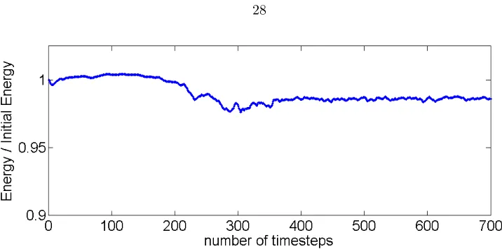
Having obtained the semidiscretization (3.21), we now wish to discretize in time. To retain good energy behavior and avoid numerical viscosity, we will use a time-symmetric discretization [17]. The lowest order time-symmetric discretizations are of order two; one may use either the trapezoidal rule or the midpoint rule. The midpoint rule has the advantage that it preserves quadratic invariants [17], including the energy of the fluid.

The trapezoidal rule, which may be derived from a variational method in the style of [43], would ordinarily give a symplectic method. However, as a rule, systems derived from a non-holonomic constraint are not symplectic unless the constraint can be rewritten to be holonomic [5]. As this is not the case for the constraint that we are using, our semidiscretization (3.21) is already not a symplectic system. Nonetheless, for completeness, we detail here how to use a discrete Lie-Poisson action to variationally derive a trapezoidal time discretization. Variational Lie-Poisson integrators have been developed before [25], but not in the presence of a non-holonomic constraint, so we derive the time integration from first principles.

The discrete action for timesteps of sizehis defined to be

Sh=

We place no restrictions on variations ofWk, and we ask that variations ofAk satisfy adiscrete Lin

on how we posit the group elementqk (denoting position of the fluid in the Lagrangian sense) to

update based on the current fluid velocity Ak. The simplest of these, which corresponds to an

explicit Euler method update of the fluid position, is

δkAk =−

Equating the variation of the action (3.29) with respect toWk to zero yields

Ak=

δH

δW(Wk), (3.31)

which, as we have seen before, is equivalent to the statementWk =dAk.

Equating the variations of the action with respect toδqk to zero fork= 1...N−1 yields

hWk−1, δkAk−1i+hWk, δkAki= 0. (3.32)

Now we substitute in the discrete Lin constraints to get

hWk−1,

where we have used the fact thatBk is antisymmetric. However, as it happensAk is also

antisym-metric, which meansAT

forAk−1, and thus,

Bk ∈ S is arbitrary, and so we find that, by the definition (3.6) of the pairing of a 2-form with a

vector field,

Recall that the semidiscretized equations were

˙

W +LAW = 0 (3.42a)

W =dA. (3.42b)

Let us examine in more detail the Lie derivative term LAW. We expand this term using the

discrete version of Cartan’s “magic” formula, which states that

LAW =diAW. (3.43)

Using the definition of the contraction (2.6), we have that, for a 2-formW and a 1-form A,

(iAW)ij =

X

m

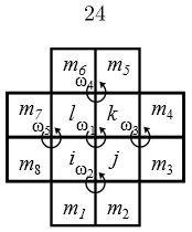
Figure 3.2: A grid for calculating the (discrete) Lie derivative.

Consider cellsiandj in Figure 3.2. Then, bearing in mind the non-holonomic constraint, we find

(iAW)ij =

X

m

(WimjAim−WjmiAjm) (3.45a)

=WiljAil+Wim1jAim1−WjkiAjk−Wjm2iAjm2. (3.45b)

Recall that if the 2-formW is equal todB[ for someB ∈ S, thenWim8j =Wjm3i= 0 (since the

cells are in a straight line), so those terms are not included above. Furthermore, this constraint onW also implies thatWilj =−Wjki. WriteWjki =ω1, and label the vorticities on other nodes

similarly (see Figure 3.2 for details). This results in the equation

(iAW)ij=−ω1(Ail+Ajk) +ω2(Aim1+Ajm2). (3.46)

Similarly, it can be calculated that

(iAW)jk=−ω1(Aji+Akl) +ω3(Ajm3+Akm4) (3.47)

(iAW)ki=ω1(Ail+Akl−Akj−Aij). (3.48)

Putting these together, the discrete form of Cartan’s formula is

(diAW)ijk= (iAW)ij+ (iAW)jk+ (iAW)ki (3.49a)

=ω2(Aim1+Ajm2) +ω3(Ajm3+Akm4). (3.49b)

Notice that, whileWijk =Wkli wheneverW =dB[ for some B ∈Ω1, it is not generally true

kliwill be the same, the update equations for these quantities will still differ. Knowing this, how can we be sure thatWijk=Wkliwill still hold at the next timestep? The answer comes from the

other equation governing the motion of the fluid, which tells us thatW =dA[_{. Given thatA has}

been restricted to satisfy the non-holonomic constraint, this places the desired restriction on the structure ofW.

We can further streamline our equations by defining the valueGijkl=Wijk+Wkli, located on

the square dual cell that overlaps with cellsi,j, kandl. Physically speaking, this is as if we have added the vorticity integrated over the triangleijkto the vorticity integrated over the trianglekli

to obtain a value integrated over the dual square ijkl. It is then natural to use linearity of the exterior derivative and define

(diAG)ijkl= (diAW)ijk+ (diAW)kli (3.50a)

=ω2(Aim1+Ajm2) +ω3(Ajm3+Akm4) (3.50b)

+ω4(Akm5+Alm6) +ω5(Alm7+Aim8). (3.50c)

This formula is nicely symmetric, and is the form that was used for the numerical results below.

3.3

Results

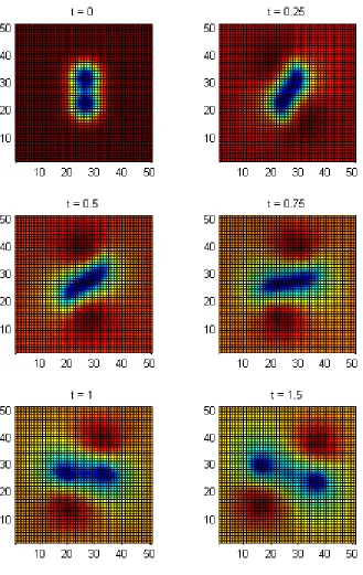
To show the good qualitative behavior of the method outlined in this chapter, we used it to simulate the behavior of two co-rotating vortices. Each vortex was given by a Gaussian vorticity distribution

ω=−a·e12

1−(x2 +y2 )

a2 , appropriately shifted away from the origin so that the two vortices start at a distanced= 0.8 apart. The width factorawas set to be 0.3. These parameters give a system that is very close to a bifurcation point. If the vortices were ever so slightly closer, they would merge. With the parameters given, however, the correct behavior should be that they move apart. Figure 3.4 shows the behavior of corotating vortex simulations using several other methods. It can be seen that methods with good energy behavior generally perform well at this test, whereas methods that introduce numerical dissipation generally cannot resolve the bifurcation point.

Figure 3.5: Energy divided by initial energy for a long-time simulation using the Hamiltonian trapezoidal method.

3.4

Discussion

The Hamiltonian methods detailed here expand our theoretical and practical understanding of the structure-preserving simulation of incompressible fluids. The spatial semi-discretization has been shown to be possible either using a continuous-time variational formalism, or using a discrete version of the Lie-Poisson bracket. We have also seen how to construct a variational Lie-Poisson time integrator in the presence of a non-holonomic constraint. We have created an energy and circulation preserving vorticity method.

In this case, because of the non-holonomic constraint, the discrete Lie-Poisson bracket does not satisfy the Jacobi identity. However, we have seen that it is nevertheless useful in the creation of a numerical method, particularly since the conservation of energy relies only on the antisymmetry of the bracket, a property which we still keep.

In the course of creating these methods, we have included the discrete codifferential, which was previously proposed by Bochev et al [6]. In combining the Hodge star with a derivative, the codifferential is sometimes more elegant than a direct Hodge star, particularly since the simplest version of the Hodge star used in DEC is the diagonal Hodge star, which is, strictly speaking, a zeroth-order approximation, whereas the codifferential based on the diagonal Hodge star may be created so as to be second-order on a regular grid, as it is essentially a central difference method.

Chapter 4

Model-Reduced Lagrangian Fluids

So far, we have seen that the technique of using a finite-dimensional Lie group to approximate the infinite-dimensional Lie group Diffvol(M) is useful for creating a semidiscretization that preserves

4.1

Derivation

We will first define the discrete, reduced scalar and velocity fields on which our functional map Lie group will act. Extending what was advocated in [10], we expand functions and vector fields using the orthonormal bases for 2-forms and 3-forms given by the eigenfunctions of the (deRham-)Laplacian operators on an arbitrary discrete meshM. These are calculated using the discrete op-erators of Finite-Element Exterior Calculus (FEEC [1]) and Discrete Exterior Calculus (DEC [11]), allowing us to leverage the large literature on their implementation and structure-preserving prop-erties with respect to topology. Although there are several sets of orthogonal eigenfunctions that we could use, this set also has the advantage of simplifying our equations in the event that we wish to add vorticity. This set of basis functions can efficiently encode through reduced coordinates the full-space fields typically used in the MAC scheme, i.e., fluxes through cell boundaries (dis-crete 2-forms) to represent velocity fields, and densities integrated in each cell (dis(dis-crete 3-forms) to represent scalar fields (such as smoke density).

4.1.1

Spectral Bases

Choice of eigenfunctions. We consider a reduced space of volume forms given by the span of the firstN Laplacian eigenfunctions on our space. To find these Laplacian eigenfunctions, we follow the approach of [10]. That is, we either calculate Laplacian eigenfunctions explicitly (in the case of a simple space like a circle or rectangle), or, more likely, we use a mesh, which need not be regular, and calculate eigenfunctions of a discrete Laplacian operator on that mesh.

We denote thei-th eigenfunction of 3-form Laplacian ∆3as Φiwith associated eigenvalue−µ2i,

∆3Φi=−µ2iΦi.

The eigenfunctions corresponding to the M3+ 1smallest eigenvalues µi can be assembled into a

low-frequency basis:

{Φ0, ...,ΦM3}.

A general volume formρwill then be represented by a vector (ρ0, ..., ρM3) of (M3+1) values, each

representing the inner product of ρ with an element of this reduced orthonormal basis, so that

ρ=PM3

than one harmonic function, but these are not influenced by divergence-free velocity fields with zero flux across the boundary and are omitted in our discussion.

Similarly, we denote the i-th eigenfunction of 2-form Laplacian ∆2 as Ψi, with its associated

eigenvalue−κ2

i:

∆2Ψi=−κ2iΨi.

We also assemble the firstM2eigenvector fields (corresponding to theM2smallest eigenvalues) into

a finite dimensional low-frequency basis:

{Ψ1, ...ΨM2}.

Some of the 2-form eigenfunctions are not divergence-free, and these eigenfunctions can be identified as gradient fields,∇Φi/µi. Thus, we can reorder the eigenfunctions of ∆2 into

{h1, ..., hβ1,

wherehiare harmonic 2-forms (corresponding to frequencyκi= 0) withβ1is the first Betti number

determined by the topology of the domain (basically, the number of tunnels plus the number of connected components of the boundary minus one), andMC=M2−M3−β1 denoting the number

of non-harmonic but divergence-free basis functions.

Lie Group action. In similar fashion to the other derivations outlined in this thesis, we represent the action of a volume-preserving diffeomorphism on the space using the approach of Koopmanism, by looking at how a given diffeomorphism acts on functions. We encode the fluid motion through a time-varying Lie group elementq(t) that represents a functional map induced by the fluid flow

φt, mapping a function f(x) =PifiΦi(x) linearly to another function g(x) =PigiΦi(x) such

thatg(x) =f◦φ−1_{(x).Since a volume form fdV is represented by a vector of (M}

3+ 1) values, a

diffeomorphismqcan be encoded by a (M3+ 1)-by-(M3+ 1) matrix.

The volume-preserving property of the flow still implies the orthogonality of the matrixq, i.e,

qt_{q= Id. So we are looking for a subgroup ofO(M}

3+1), or, more accurately, of SO(M3+1), since

we wish to describe gradual changes from the identity.

becomesq0i=δ0i andqi0=δi0, whereδij is the Kronecker symbol, since 0-th frequency represents

the constant function. This effectively removes one dimension of possible changes that an element of the Lie group could make. The Lie group that we are using is thus isomorphic to SO(M3).

This is much smaller than the full Lie group used for the spatial representation [32], which had a dimension proportional to the square of the number of cells of the mesh—a potential reduction of several orders of magnitude.

Lie Algebra. We identify each velocity eigenfunction Ψm with an element of the Lie algebra of

the above Lie group as follows. We take the Lie derivative along the velocity field Ψm of a scalar

eigenfunction Φi projected onto another scalar eigenfunction Φj, which is a matrix Am for each

velocity eigenfunction Ψm, with entries

Am,ij =

Z

M

Φi(Ψm· ∇Φj). (4.1)

As in the non-spectral case, the divergence-free condition leads to the antisymmetry of these ma-trices:

This is expected, since the Lie algebra so(M3) ofSO(M3) contains only antisymmetric matrices.

The Lie algebra has a Lie bracket given by the usual matrix commutator [Am, An] =AmAn−AnAm.

4.1.2

Non-holonomic constraint.

There areM3(M3−1)/2 degrees of freedom in the Lie algebra of antisymmetric matricesso(M3).

However, we cannot simply use the first M3(M3−1)/2 elements of the Laplacian basis of vector

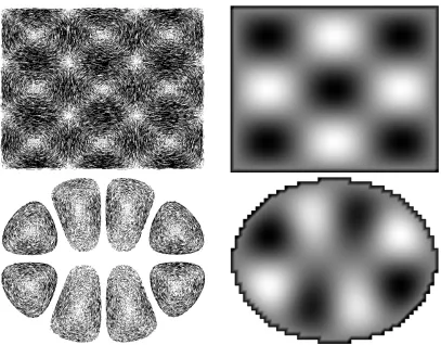
Figure 4.1: Effect of shape on spectral bases: The Laplacian eigenvectors depends heavily on the domain Ω. Here, rectangle (top) vs. ellipse (bottom) domains (both computed on 2D rectangular grid of size 1202_{) exhibit very different eigenvectors Ψ}

still of such high frequency that its inner product with each basis element Φigives zero. The space

of divergence-free vector fields acting on the reduced basis of volume forms is of lower dimension than the Lie algebra. It follows that some elements of the Lie algebra must not correspond to a vector field at all.

We force the dynamics on the Lie algebra to remain within the domain of physically-sensible elements using the following non-holonomic constraint, which keeps the velocity within the space spanned by the lowest frequencyMC+β1 divergence-free 2-form basis fields:

A=

MC+β1 X

i=1

viAi (4.3)

where vi is a coefficient for Ai representing the modal amplitude of frequency κi. This linear

condition can be seen as an intuitive extension of the one-away spatial constraint on Lie algebra elements that was used in [32] and explained in Section 2.2.3. Instead of constraining interactions to be local in space, we have constrained them to the part of the Lie algebra that corresponds to lower-frequency basis functions1.

4.1.3

Implementation

Computing our spectral bases requires a proper discretization of the Laplacian operators and of boundary conditions. Both topics are well studied, and many implementations can be leveraged [12, 4]. A detailed guide to discretization onarbitrary unstructured meshesmay be found in Appendix A of [23] to explicate how to enforce no-transfer and free-slip conditions (corresponding, respectively, tovn|∂M= 0 and∂vt/∂n|∂M= 0 if the continuous velocity field is decomposed at the boundary into

its normal and tangential components,v=vn+vt). Note that only two operators are required: the

exterior derivativedand the Hodge star?. The first operator is purely topological, while the second is just a scaling operation per edge, face, and cell. Moreover, as explained in the next paragraph, this latter operator can be trivially modified to handle arbitrary fluid domains without having to use anything else but a regular grid. From these two operators, both Laplacians are easily assembled, and low-frequency eigenfields are found via Lanczos iterations since each operator is symmetric by construction.

Figure 4.3: Domain-altered Hodge stars: Hedge-hog visualization of Ψ5on a 2562grid for three

different 2D domain shapes, obtained through a simple alteration of the Hodge star? operator.

To implement embedded boundaries we propose a simple extension of the technique of [30] to computek-form Laplacians of an arbitrary domainwhile still using a regular grid. This renders the implementation of Laplacians and their boundary conditions quite trivial, and removes the arduous task of tetrahedralizing arbitrary domains. This idea was introduced in [3] for their pressure-based projection, and a simple alteration proposed by [30] made the approach robust and convergent. We leverage this latter work by noticing that the modification of the Laplacian ∆3that they proposed

amounts to a local change to the Hodge star operator?2.

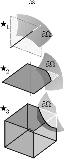
More precisely, consider a continuous domain Ω, e.g., defined implicitly by a function χ via Ω ={x|χ(x)≥0} (see Figure 4.4). Recall that the diagonal Hodge stars on a mesh M are all expressed using local ratios of measurements (edge lengths, face areas, cell volumes) on both the primal elements ofMand its dual elements [11]. The changes to the Laplacian operator ∆3that Ng

et al. [30] introduced can be reexpressed by an alteration of the Hodge star?2, whereeach primal

area measurement only counts the part of the primal face that is inside Ω, but dual edge lengths are kept unchanged. We extend this simple observation (which amounts to a local, numerical homogenization to capture sub-grid resolution) by computing modified Hodge stars ˆ?1,ˆ?2, and ˆ?3

Figure 4.4: Diagram of the Hodge star near an embedded boundary.

behavior of this Hodge star modification under refinement of the regular grid for a given continuous elliptic domain Ω, resulting in very good approximations of the eigenvectors.

4.1.4

Spectral variational integrator

The Lagrangian of the fluid motion (i.e., its kinetic energy in the case of Euler fluids) can be written asLEuler=

1

2hA(t), A(t)ias we reviewed in Sec. 2.3. Thus, the equation of motion can be derived

from Hamilton’s (least action) principle:

Z

hA(t), δAidt= 0 (4.4)

under the Lin constraint [14] restricting the variations ofAto those of the form

Figure 4.5: Convergence of Laplacians: Our discretization of the two Laplacians creates (vector and scalar) eigenfields that converge under refinement of the regular grid used to compute them, extending the linear convergence proved in [30]. Here, particle-tracing visualization of the 15th eigenbasis for vector fields on the ellipse (top) at resolution 302, 602, 1202, and 2402, and 15theigen function (bottom) at the same resolutions.

whereB=P

iξiAi is an arbitrary element of the Lie algebra with coordinates{ξi}i in the 2-form

basis. Substituting Eq.(4.5) into Eq.(4.4), we then have

0 =

Since this last equation must be valid for anyξk, the update rule for the velocity field has to be

˙

vk =

X

i,j

vivjhAi,[Aj, Ak]i ≡vTCkv, (4.6)

wherevis the column vector storing the coefficientsviof the discrete velocityA(Eq. 4.3), and Ck

is the square matrix with components

Ck,ij =hAi,[Aj, Ak]i=

Z

M

Time integrator. The continuous-time update in Eq. 4.6 is then discretized via either a midpoint rule (which will lead to an energy-preserving model-reduced variant of [28]) or a trapezoidal rule (which corresponds to a model-reduced variant of the variational method of [32]). Specifically, the midpoint rule is implemented as

The energy preservation can be easily verified by multiplyingvt_k+vt_k+h on both sides of the above equation, summing overk, and invoking the property of coefficientsCk,ij=−Cj,ik. The trapezoidal

rule can, instead, be implemented as

vt_k+h−v_kt =h

which is derived from a temporal discretization of the action with variation of (δq)q−1_{forqalong the}

path to be in the restricted Lie algebra set (to enforce Lin constraints). Both the energy-preserving and trapezoidal variational method are time-reversible implicit methods solved through a simple quadratic set of equations with a small number of variables. Note that an explicit forward Euler integration can also be used for small time steps, but with no guarantee of good behavior over long periods of time.

4.1.5

Kelvin’s circulation theorem

The model-reduced method obeys a form of Kelvin’s theorem as follows. We can define generalized curves as spectral dual 1-chains (also called 1-currents [11]) of the form:

Γ =X

i

γi?2Ai. (4.10)

is boundaryless. A pairing between a 2-form and a generalized loop is defined as expected:

The Lie advection of the generalized curve along the velocity field

˙

Γ =−[A,Γ] (4.12)

indicates that the coefficients{γi}i must evolve such that

˙

Thus, the spectral version of Kelvin’s theorem holds since

d

In the above derivation, dummy index variables are swapped and the identity Ck,ij = −Cj,ik is

used.

4.2

Results

All these results are taken from [23], with thanks to Beibei Liu and Julian Hodgson for the images, and were generated on an Intel i7 laptop with 12GB RAM.

initial velocity field at timet= 0 that only contains non-zero components for the first 120 frequencies. We then advected the fluid using our integrator, with fluid markers initially set as two colored disks near the center. Because of the propensity of vorticity to go to higher scales, our reduced approach does not lead to the exact same position of the fluid markers after 12s of simulation if one uses only 120 bases. However, as the number of bases increases to 300 or 500, the simulation quickly captures the same dynamical behavior as a full variational integrator with 2562degrees of freedom (see Figure 4.6).

Figure 4.6: Convergence of simulation: A flow in a periodic domain is initialized with a band-limited velocity fields with 120 wave number vectors. Fluid markers (forming a blue and red circle) are added for visualization. After 12s of simulation, the results of our reduced approach (from the left: with 120,300, 500 modes) vs. the full 2562 _{dynamics (right) are qualitatively similar.}

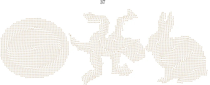
Figure 4.7:Model-reduced fluids on regular grids. Our energy-preserving approach integrates a fluid flow variationally using a small number of divergence-free velocity field bases over an arbitrary domain (visualized here are the 5th_{, 10}th_{, and 15}th_{eigenvectors of the 2-form Laplacian) computed}

with subgrid accuracy on a regular grid (here, a 42×42×32 grid). Our integrator is versatile: it can be used for realtime fluid animation, magnetohydrodynamics, and turbulence models, with either explicit or implicit integration.

Advanced fluid models. We also extended our method to the LANS-α turbulence model to better capture the spectral energy distribution with a small number of modes. On a 3D regular grid, we performed a simulation as described in [13] by holding the low wave number componentsvi

fixed for|κi|<2 to act as a forcing term, and running the simulation untilt= 100. We then extracted the average spectral energy distribution present between t= 33 to t= 100. We show in Fig. 4.12 that the Kolmogorov “−5/3 law” is much better captured than with the usual Navier-Stokes model, even for the low number of modes used in our spectral context: theα-model produces a decay rate at high wave numbers much steeper than a Navier-Stokes simulation, allowing us to cut off the higher frequencies at a lower threshold without significant deviation from the spectral distribution. This indicates that our approach consisting in a simple scaling of the structural coefficients helps improving fluid simulation on coarse grids.

full-Figure 4.8: Robustness to resolution: With the homogenized boundary condition on grids of resolution 402 _{(blue), 80}2 _{(green), and 160}2 _{(red), no staircase artifacts are observed, and the}

simulation results are consistent across resolutions.

blown 1282 _{grid takes around 50s for the variational integrator to update one step (through a}

Newton solver) in a typical simulation using the trapezoidal rule update, while a 50-mode (resp., 100-mode and 200-mode) simulation with our integrator takes only 0.098s (resp., 0.65s and 2.0s) for complex boundaries (i.e., with dense structural coefficients), and 0.026s (resp., 0.070s, 0.28s) for simple box domains (with sparse coefficients). Our Newton solver normally converges in a couple of iterations depending on the time step size (which determines the quality of the initial guess); for instance, the average in our 3D bunny buoyancy test in Fig. 4.2 is below 3 iterations. Depending on how many modes the user is willing to discard (and replace by wavelet noise or dynamical texture for efficiency), the computational gains can thus total several orders of magnitude, and this allows us to simulate flows at interactive rates—or even in realtime for periodic 3D domains if we compute the eigenbases in closed form as shown in Fig. 4.11. Note however that our model-reduced integrator suffers from the usual limitation of model reduction: the complexity is actually growing quadratically (resp., cubically) with the number of modes for sparse (resp., dense) structural coefficients. So our integrator is numerically efficient only for relatively low mode counts.

4.2.1

Generalization to other bases

of scalar basis elements Φi (orthonormalized through the Gram-Schmidt procedure) and a set of

velocity basis elements Ψi. The Lie derivative matrixAwill still be antisymmetric as long as Ψi’s

are divergence-free. This means that one can use existing finite element basis functions instead of our Laplace eigenvectors—or even wavelet bases ofH(div,Ω) (see for instance [42]) if spatially localized basis functions are sought after to get a sparser advection. The key to the numerical benefits of our variational approach is to ensure the anti-commutativity of the Lie bracket in the evaluation of hAi,[Aj, Ak]i (Eq. (4.7)) and the advection of other fields by the exponential map

Figure 4.9: Curved domain: While all our other results were achieved on a regular grid, our approach applies to arbitrary domains, here on the surface of a triangulated domain; a simple laminar flow with initial horizonal velocity smoothly varying along the vertical direction quickly develops vortical structures on this complex surface.

Figure 4.11: Interactivity: We can also use the analytic expressions for Ψk andCk,ijin a periodic

3D domain to handle a large number of modes without even calculating the spectral bases. The explicit update rule exhibits no artificial damping of the energy as expected, but offers realtime flows.

4.3

Discussion

We have introduced a variational integrator for fluid simulation in reduced coordinates. By restrict-ing the variations in Hamilton’s principle to a low-dimensional space spanned by low-frequency divergence-free velocity fields, our method exhibits the properties of variational integrators in cap-turing the qualitatively correct behavior of ideal incompressible fluids (such as Kelvin’s circulation and energy preservation) while greatly reducing the computational cost. The resulting method is versatile, energy-preserving, and computationally efficient.

While any application targeting low computational complexity of fluid simulation will benefit from this reduced space approach, one possible limitation of our method in some cases is the lack of spatial locality in our bases. For this reason, it should be noted that our integrator is not restricted to a particular set of basis functions. Future work could explore the use of wavelets for vorticity to offer optimal sparsity in the structural coefficients. Another possible future extension is to incorporate free surface boundary conditions through our modified Hodge star, combined with wavelet representations for the volume of fluid per cell.

4.3.1

Persistence of non-holonomic constraints

Among the initial aims for this method was the hope that the use of a reduced basis would allow us to forgo the non-holonomic constraint used in earlier methods [32]. This proved impossible, because the mapping that we chose between Laplacian basis functions for the vector field and the Lie algebra

gwas not surjective, and thus there were elements of the Lie algebra that did not correspond to any vector field.

A related problem is that the Lie bracket is not preserved by this form of discretization. Instead, taking Lie brackets in the continuous space leads us to higher-frequency functions, which would require more basis functions if we wished to resolve them. This tendency of the Lie bracket to lead us outside our reduced basis is related to the cascade of energy to higher-frequency motions, as famously recognized by Kolmogorov [20]. In theory, if we could find a set of finite-dimensional Lie algebra discretizations which did preserve the Lie bracket, this problem could be solved. In particular, this would require a Lie algebra isomorphic to a suitable finite-dimensional Lie subalgebra of χvol. I have not found in the literature any complete classification of finite-dimensional Lie

would probably have been noted before now.

Chapter 5

Spectral Discrete Exterior

Calculus

We have seen that we can create a Lie group based method for incompressible fluids using Laplacian eigenfunctions, and this method may be easily extended to other sets of orthogonal eigenfunctions. We have also seen that the Lie group method for fluids has limitations, because it requires the non-holonomic constraint, which breaks the symplecticity of the method. One possible avenue for future work is to try to find a structured integrator for fluids using a field theoretic perspective rather than the Lie group perspective. For this purpose, it may be useful to build on work I did with Dzhelil Rufat, Patrick Mullen, and my adviser on a spectral version of discrete exterior calculus.

Discrete exterior calculus [11] represents k-forms by integrating them on k-dimensional elements of a mesh. Thus, 0-forms are represented by their values at points, 1-forms are represented by quantities integrated along edges, 2-forms on faces, and 3-forms on volumes. One particularly nice aspect of this style of discretization is that we can use Stokes’ theorem to define a discrete exterior derivative which introducesno error whatsoever– see Section 5.2.1. Along with this discrete exterior derivative, we define operators of discrete exterior calculus such as the wedge product and the hodge star. These operatorsdo introduce error. In particular, existing versions are sometimes of very low order. For example, the diagonal hodge star is zeroth order [11].

us to take into account the fact that we are dealing with integrated quantities, which is an essential element in preserving the perfect accuracy of the discrete exterior derivative. We may then apply the corresponding continuous operator to the interpolated or histopolated function, before discretizing again using areduction operator. In this way we are able to create a spectrally-accurate discrete exterior calculus.

5.1

Basic Spectral Tools

Before delving into the design of spectrally-accurate discrete operators, we must define a series of basic tools and conventions which will be particularly useful for our task. We start by introducing the general notions of reduction and reconstruction maps. The reduction map will allow us to represent a continuous form in terms of a finite number of basis functions. The reconstruction map will then allow us to reconstruct the continuous form again from this information.

The reduction and reconstruction maps will first be explained in terms of general basis functions. We will then proceed to define the spectral basis functions on periodic regular grids which our specific reduction and reconstruction maps will use, before moving on to the case of Chebyshev grids, which allow us to consider regions with boundaries.

5.1.1

Reduction and Reconstruction Maps

The reduction and reconstruction maps provide a way to go back and forth between continuous forms and their discrete realizations.

Reduction. The reduction map (also called the de Rham map) is a linear operatorPthat projects a continuous form to its discrete realization on the grid through integration over mesh elements:

P: Λk→Λ¯k

ωk →ω¯k with ω¯ik= (Pω k

)i≡

Z

σk i

We will denote by Pe the analogous operator mapping continuous forms to their dual discrete

Note that this definition of reduction extends the notion ofpoint sampling: while the reduction of a 0-form is found by simply point-sampling its value at each vertex of the grid, the reduction of a generalk-form is its evaluation (i.e., integral) on all thek-dimensional elements (vertices fork= 0, edges fork= 1, faces fork= 2, etc) of the grid.

Reconstruction. Conversely, the reconstruction map (R) is a map which reconstructs a contin-uousk-form from its discrete realization by interpolation fork= 0, and by histopolation otherwise:

R: Λ¯k →Λk

¯

ωk→ωk.

We will denote byRe the analogous operator mappingdual discrete forms to continuous forms in a

similar fashion. Note that we will sometimes omit the dual sign_e.for clarity, as which reconstruction operator is meant is unambiguously implied by the (primal or dual) nature of the discrete form it is applied on.

then,Rcan trivially be defined as

ωk=Rω¯k ≡X i

¯

One can readily verifies that this reduction map is a left inverse of the reconstruction map:

PR= Id.

However, the converse is not true; the reconstruction map is only approximately the right inverse of the reduction map, with equality in the limit when the mesh element sizehapproaches 0:

kω− RPωk −−−→ h→0 0,

with a rate of convergence determined by the chosen norm on forms and the degree of the basis functions. While Whitney first introduced a one-sided inverse of the de Rham map using what amounts to piecewise linear basis functions [44], we will instead use global basis functions satisfying Eq. (5.1) to provide spectrally-accurate reconstructions.

5.1.2

1D Periodic Interpolator & Histopolator Functions

To build our spectral wedge and Hodge star operators to work on discrete forms