An Improved Hierarchical Bayesian Model of Language for Document Classification

(1)

An Improved Hierarchical Bayesian Model of Language

for Document Classification

Ben Allison

Department of Computer Science University of Sheffield

UK

Abstract

This paper addresses the fundamental problem of document classification, and we focus attention on classification prob-lems where the classes are mutually exclu-sive. In the course of the paper we advo-cate an approximate sampling distribution for word counts in documents, and demon-strate the model’s capacity to outperform both the simple multinomial and more re-cently proposed extensions on the classifi-cation task. We also compare the classi-fiers to a linear SVM, and show that pro-vided certain conditions are met, the new model allows performance which exceeds that of the SVM and attains amongst the very best published results on the News-groups classification task.

1 Introduction

Document classification is one of the key technolo-gies in the emerging digital world: as the amount of textual information existing in electronic form increases exponentially, reliable automatic meth-ods to sift through the haystack and pluck out the occasional needle are almost a necessity.

Previous comparative studies of different classi-fiers (for example, (Yang and Liu, 1999; Joachims, 1998; Rennie et al., 2003; Dumais et al., 1998)) have consistently shown linear Support Vector

Ma-chines to be the most appropriate method.

Gen-erative probabilistic classifiers, often represented

by the multinomial classifier, have in these same

studies performed poorly, and this empirical evi-dence has been bolstered by theoretical arguments (Lasserre et al., 2006).

In this paper we revisit the theme of genera-tive classifiers for mutually exclusive classification problems, but consider classifiers employing more complex models of language; as a starting point we consider recent work (Madsen et al., 2005) which relaxes some of the multinomial assump-tions. We continue and expand upon the theme of that work, but identify some weaknesses both in its theoretical motivations and practical applica-tions. We demonstrate a new approximate model which overcomes some of these concerns, and demonstrate substantial improvements that such a model achieves on four classification tasks, three of which are standard and one of which is a newly created task. We also show the new model to be highly competitive to an SVM where the previous models are not.

§2 of the paper describes previous work which has sought a probabilistic model of language and its application to document classification. §3 de-scribes the models we consider in this paper, and gives details of parameter estimation. §4 describes our evaluation of the models, and §5 presents the results of this evaluation. §6 explores reasons for the observed results, and finally §7 ends with some concluding remarks.

2 Related Work

The problem of finding an appropriate and tractable model for language is one which has been studied in many different areas. In many cases, the first (and often only) model is one in which counts of words are modelled as binomial– or Poisson– distributed random variables. However, the use of such distributions entails an implicit assumption

(2)

that the occurrence of words is the result of a fixed number of independent trials—draws from a ”bag of words”—where on each trial the probability of success is constant.

Several authors, among them (Church and Gale, 1995; Katz, 1996), observe empirically such mod-els are not always accurate predictors of actual word behaviour. This moves them to suggest dis-tributions for word counts where the underlying probability varies between documents; thus the ex-pected behaviour of a word in a new document is a combination of predictions for all possible prob-abilities. Other authors (Jansche, 2003; Eyhera-mendy et al., 2003; Lowe, 1999) use these same ideas to classify documents on the basis of subsets of vocabulary, in the first and third cases with en-couraging results using small subsets (in the sec-ond case, the performance of the model is shown to be poor compared to the multinomial).

When one moves to consider counts of all words in some vocabulary, the proper distribution of the whole vector of word counts is multinomial. (Madsen et al., 2005) apply the same idea as for the single word (binomial) case to the multino-mial, using the most convenient form of distribu-tion to represent the way the vector of multino-mial probabilities varies between documents, and report encouraging results compared to the simple multinomial. However, we show that the use of the most mathematically convenient distribution to describe the way the vector of probabilities varies entails some unwarranted and undesirable tions. This paper will first describe those assump-tions, and then describe an approximate technique for overcoming the assumptions. We show that, combined with some alterations to estimation, the models lead to a classifier able to outperform both the multinomial classifier and a linear SVM.

3 Probabilistic Models of Language for Document Classification

In this section, we briefly describe the use of a gen-erative model of language as applied to the prob-lem of document classification, and also how we estimate all relevant parameters for the work which follows.

In terms of notation, we usec˜to represent a

ran-dom variable andc to represent an outcome. We

use roman letters for observed or observable quan-tities and greek letters for unobservables (i.e.

pa-rameters). We writec˜∼ ϕ(c)to mean that ˜chas

probability density (discrete or continuous) ϕ(c),

and writep(c)as shorthand forp(˜c= c). Finally,

we make no explicit distinction in notation be-tween univariate and multivariate quantities;

how-ever, we useθj to refer to thej-th component of

the vectorθ.

We consider documents to be represented as vectors of count–valued random variables such

that d = {d1...dv}. For classification, interest

centres on the conditional distribution of the class variable, given such a document. Where docu-ments are to be assigned to one class only (as in the case of this paper), this class is judged to be the most probable class. For generative classifiers such as those considered here, the posterior bution of interest is modelled from the joint

distri-bution of class and document; thus ifc˜is a variable

representing class andd˜is a vector of word counts,

then:

p(c|d)∝p(c)·p(d|c) (1) For the purposes of this work we also assume a

uniform prior on˜c, meaning the ultimate decision

is on the basis of the document alone.

Multinomial Sampling Model

A natural way to model the distribution of

counts is to letp(d|c)be distributed multinomially,

as proposed in (Guthrie et al., 1994; McCallum and Nigam, 1998) amongst others. The multino-mial model assumes that documents are the result of repeated trials, where on each trial a word is se-lected at random, and the probability of selecting

thej-th word from classcisθcj. However, in

gen-eral we will not use the subscriptc– we estimate

one set of parameters for each possible class.

Using multinomial sampling, the term p(d|c)

has distribution:

pmultinomial(d|θ) = P

jdj

!

Q j(dj!)

Y

j θdj

j (2)

A simple Bayes estimator forθcan be obtained

by taking the prior forθas a Dirichlet distribution,

in which case the posterior is also Dirichlet. De-note the total training data for the class in

ques-tion as D = {(d11...d1v)...(dk1...dkv)} (that is,

counts of each ofvwords inkdocuments). Then

ifp(θ)∼Dirichlet(α1...αv), the mean ofp(θ|D)

for thej-th component ofθ(which is the estimate

(3)

ˆ

θj = E[θj|D] = Pαj+nj

jαj+n• (3)

where thenj are the sufficient statisticsP_inij,

andn•isPjnj. We follow common practice and

use the standard reference Dirichlet prior, which is

uniform onθ, such thatαj = 1for allj.

3.1 Hierarchical Sampling Models

In contrast to the model above, a hierarchical

sam-pling model assumes thatθ˜varies between

docu-ments, and has distribution which depends upon

parameters η. This allows for a more realistic

model, letting the probabilities of using words vary between documents subject only to some general trend.

For example, consider documents about politics: some will discuss the current British Prime Minis-ter, Gordon Brown. In these documents, the

proba-bility of using the wordbrown(assuming case

nor-malisation) may be relatively high. Other politics articles may discuss US politics, for example, or the UN, French elections, and so on, and these ar-ticles may have a much lower probability of using

the wordbrown: perhaps just the occasional

refer-ence to the Prime Minister. A hierarchical model attempts to model the way this probability varies between documents in the politics class.

Starting with the joint distributionp(θ, d|η)and

averaging over all possible values thatθmay take

in the new document gives:

p(d|η) =

ˆ

p(θ|η)p(d|θ)dθ (4)

where integration is understood to be over the

entire range of possible θ. Intuitively, this allows

˜

θto vary between documents subject to the

restric-tion thatθ˜∼p(θ|η), and the probability of

observ-ing a document is the average of its probability for

all possibleθ, weighted byp(θ|η). The sampling

process is 1) θ is first sampled from p(θ|η) and

then 2) dis sampled from p(d|θ), leading to the

hierarchical name for such models.

Dirichlet Compound Multinomial Sampling Model

(Madsen et al., 2005) suggest a form of (4)

where p(θ|η) is Dirichlet-distributed, leading to

aDirichlet–Compound–Multinomialsampling

dis-tribution. The main benefit of this assumption is that the integral of (4) can be obtained in closed

form. Thusp(d|α)(using the standardα notation

for Dirichlet parameters) has distribution:

pDCM(d|α) = P

jdj

!

Q

j(dj!) ×

ΓP_jαj

ΓP_jdj+αj

×Y

j

Γ(αj +dj)

Γ(αj) (5)

Maximum likelihood estimates for theαare

dif-ficult to obtain, since the likelihood forαis a

func-tion which must be maximised for all components simultaneously, leading some authors to use ap-proximate distributions to improve the tractability of maximum likelihood estimation (Elkan, 2006). In contrast, we reparameterise the Dirichlet com-pound multinomial, and estimate some of the pa-rameters in closed form.

We reparameterise the model in terms ofµand

λ – µ is a vector of length v, and λ is a

con-stant which reflects the variance ofθ. Under this

parametrisation,αj = λµj. The estimate we use

forµjis simply:

ˆ

µj = n_nj

• (6)

wherenjandn•are defined above. This simply

matches the first moment about the mean of the distribution with the first moment about the mean of the sample. Once again letting:

D={d1...dk}={(d11...d1v)...(dk1...dkv)}

denote the training data such that thediare

indi-vidual document vectors anddij are counts of the

j-th word in the i-th document, the likelihood for

λis:

L(λ) =Y

i

Γ(P_jλµj)

Γ(P_jdij +λµj) Y

j

Γ(λµj +dij)

Γ(λµj)

(7) This is a one–dimensional function, and as such is much more simple to maximise using standard optimisation techniques, for example as in (Minka, 2000).

As before, however, simple maximum likeli-hood estimates alone are not sufficient: if a word

fails to appear at all in D, the corresponding µj

(4)

to incorporate a prior on either α or (under our

parameterisation) µ; however, this would lead to

high computational cost as the resulting posterior would be complicated to work with. (Madsen et

al., 2005) instead set eachαˆjas the maximum

like-lihood estimate plus some , in some ways

echo-ing the estimation ofθfor the multinomial model.

Unfortunately, unlike a prior this strategy has the same effect regardless of the amount of training data available, whereas any true prior would have diminishing effect as the amount of training data increased. Instead, we supplement actual training data with a pseudo–document in which every word occurs once (note this is quite different to setting

= 1); this echoes the effect of a true prior onµ,

but without the computational burden.

A Joint Beta-Binomial Sampling Model

Despite its apparent convenience and theoretical well–foundedness, the Dirichlet compound multi-nomial model has one serious drawback, which is emphasised by the reparameterisation. Under the Dirichlet, there is a functional dependence

be-tween the expected value ofθj,µjand its variance,

where the relationship is regulated by the constant

λ. Thus two words whoseµjare the same will also

have the same variance in theθj. This is of concern

since different words have different patterns of use – to use a popular turn of phrase, some words are more “bursty” than others (see (Church and Gale, 1995) for examples). In practice, we may hope to model different words as having the same ex-pected value, but drastically different variances – unfortunately, this is not possible using the Dirich-let model.

The difficulty with switching to a different model is the evaluation of the integral in (4). The integral is in fact in many thousands of dimensions, and even if it were possible to evaluate such an integral numerically, the process would be excep-tionally slow.

We overcome this problem by decomposing the

term p(d|η) into a product of independent terms

of the form p(dj|ηj). A natural way for each of

these terms to be distributed is to let the probability

p(dj|θj) be binomial and to letp(θj|ηj)be beta–

distributed. The probabilityp(dj|ηj)(whereηj =

{αj, βj}, the parameters of the beta distribution) is

then:

pbb(dj|αj, βj) =

n dj

B(dj+αj, n−dj+βj)

B(αj, βj)

(8)

where B(•) is the Beta function. The term

p(d|η)is then simply:

pbeta−binomial(d|η) = Y

j

p(dj|ηj) (9)

This allows means and variances for each of the

θj to be specified separately, but this comes at a

price: while the Dirichlet ensures thatP_jθj = 1

for all possibleθ, the model above does not. Thus

the model is only an approximation to a true model

where components of θ have independent means

and variances, and the requirements of the multi-nomial are fulfilled. However, given the inflexibil-ity of the Dirichlet multinomial model, we argue that such a sacrifice is justified.

In order to estimate parameters of the Beta– Binomial model, we take a slight departure from both (Lowe, 1999) and (Jansche, 2003) who have both used a similar model previously for individual words. (Lowe, 1999) uses numerical techniques

to find maximum likelihood estimates of the αj

andβj, which was feasible in that case because of

the highly restricted vocabulary and two-classes. (Jansche, 2003) argues exactly this point, and uses moment–matched estimates; our estimation is sim-ilar to that, in that we use moment–matching, but different in other regards.

Conventional parameter estimates are affected (in some way or other) by the likelihood function for a parameter, and the likelihood function is such that longer documents exert a greater influence on the overall likelihood for a parameter. That is, we

note that if the true binomial parameterθij for the

j-th word in thei-th document were known, then

the most sensible expected value for the

distribu-tion overθjwould be:

E [θj] = _k1 × k X

i=1

θij (10)

Whereas the expected value of conventional method–of–moments estimate is:

E [θj] = k X

i=1

p(θij)×θˆij (11)

That is, a weighted mean of the maximum

(5)

given byp(θij), i.e. the length of the i-th

docu-ment. Similar effects would be observed by max-imising the likelihood function numerically. This is to our minds undesireable, since we do note be-lieve that longer documents are necessarily more representative of the population of all documents than are shorter ones (indeed, extremely long doc-uments are likeliy to be an oddity), and in any case the goal is to capture variation in the parameters.

This leads us to suggest estimates for parameters such that the expected value of the distribution is

as in 10 but with theθij (which are unknown)

re-placed with their maximum likelihood estimates,

ˆ

θij. We then use these estimates to specify the

de-sired variance, leading to the simultaneous equa-tions:

αj αj+βj =

P iθˆij k (12) αjβj

(αj +βj)2(αj+βj+ 1) = P

i(ˆθij −E[θj])2

k (13)

As before, we supplement actual training doc-uments with a pseudo-document in which every

word occurs once to prevent anyαjbeing zero.

4 Evaluating the Models

This section describes evaluation of the models above on four text classification problems.

The Newsgroups task is to classify postings into one of twenty categories, and uses data originally collected in (Lang, 1995). The task involves a rel-atively large number of documents (approximately 20,000) with roughly even distribution of mes-sages, giving a very low baseline of approximately 5%.

For the second task, we use a task derived from the Enron mail corpus (Klimt and Yang, 2004), de-scribed in (Allison and Guthrie, 2008). Corpus is a nine–way email authorship attribution problem, with 4071 emails (between 174 and 706 emails per

author)1_{. The mean length of messages in the}

cor-pus is 75 words.

WebKB is a web–page classification task, where the goal is to determine the webpage type of the unseen document. We follow the setup of (McCal-lum and Nigam, 1998) and many thereafter, and

1_{The corpus is available for download from} www.dcs.shef.ac.uk/˜ben.

use the four biggest categories, namelystudent,

faculty,courseandproject. The resulting corpus consists of approximately 4,200 webpages. The SpamAssassin corpus is made available for public use as part of the open-source Apache

Spa-mAssassin Project2_{. It consists of email divided}

into three categories: Easy Ham, which is email

unambiguously ham (i.e. not spam), Hard Ham

which is not spam but shares many traits with

spam, and finallySpam. The task is to apply these

labels to unseen emails. We use the latest ver-sion of all datasets, and combine the easy ham and easy ham 2 as well as spam and spam 2 sets to form a corpus of just over 6,000 messages.

In all cases, we use 10–fold cross validation to make maximal use of the data, where folds are chosen by random assignment. We define “words” to be contiguous whitespace–delimited alpha–numeric strings, and perform no stemming or stoplisting.

For the purposes of comparison, we also present results using a linear SVM (Joachims, 1999), which we convert to multi–class problems using a one–versus–all strategy shown to be amongst the best performing strategies (Rennie and Rifkin, 2001). We normalise documents to be vectors of unit length, and resolve decision ambiguities by sole means of distance to the hyperplane. We also note that experimentation with non–linear kernels showed no consistent trends, and made very little difference to performance.

[image:5.595.98.292.311.397.2]

5 Results

Table 1 displays results for the three models over the four datasets. We use the simplest measure of classifier performance, accuracy, which is simply the total number of correct decisions over the ten folds, divided by the size of the corpus. In response to a growing unease over the use of significance tests (because they have a tendency to overstate significance, as well as obscure effects of sample size) we provide 95% intervals for accuracy as well as the metric itself. To calculate these, we view ac-curacy as an (unknown) parameter to a binomial distribution such that the number of correctly clas-sified documents is a binomially distributed ran-dom variable. We then calculate the Bayesian in-terval for the parameter, as described in (Brown et al., 2001), which allows immediate quantification

(6)

of uncertainty in the true accuracy after a limited sample.

As can be seen from the performance figures, no one classifier is totally dominant, although there are obvious and substantial gains in using the Beta-Binomial model on the Newsgroups and Enron tasks when compared to all other models. The Spa-mAssassin corpus shows the beta–binomial model and the SVM to be considerably better than the other two models, but there is little to choose be-tween them. The WebKB task, however, shows extremely unusual results: the SVM is head and shoulders above other methods, and of the genera-tive approaches the multinomial is clearly superior. In all cases, the Dirichlet model actually performs worse than the multinomial model, in contrast to the observations of (Madsen et al., 2005).

In terms of comparison with other work, we note that the performance of our multinomial model agrees with that in other work, including for exam-ple (Rennie et al., 2003; Eyheramendy et al., 2003; Madsen et al., 2005; Jansche, 2003). Our Dirichlet model performs worse than that in (Madsen et al., 2005) (85% here compared to 89% in that work), which we attribute to their experimentation with

alternate smoothing as described in §3.1. We

note however that the Beta-Binomial model here still outperforms that work by some considerable margin. Finally, we note that our beta–binomial model outperforms that in (Jansche, 2003), which we attribute mainly to the altered estimate, but also to the partial vocabulary used in that work. In fact, (Jansche, 2003) shows there to be little to sepa-rate the beta-binomial and multinomial models for larger vocabularies, in stark contrast to the work here, and this is doubtless due to the parameter es-timation.

6 Analysis

One might expect performance of a hierarchical sampling model to eclipse that of the SVM because of the nature of the decision boundary, provided certain conditions are met: the SVM estimates a linear decision boundary, and the multinomial classifier does the same. However, the decision boundaries for the hierarchical classifiers are non– linear, and can represent more complex word be-haviour, provided that sufficient data exist to pre-dict it. However, unlike generic non–linear SVMs (which made little difference compared to a lin-ear SVM) the non–linlin-ear decision boundary here

arises naturally from a model of word behaviour. For the hierarchical models, performance rests on the ability to estimate both the rate of word

oc-currence θj and also the way that this rate varies

between documents. To reliably estimate variance (and arguably rate as well) would require words to occur a sufficient number of times. However, this section will demonstrate that two of the datasets have many words which do not occur with suf-ficient frequency to estimate parameters, and in those two the linear SVM’s performance is more comparable.

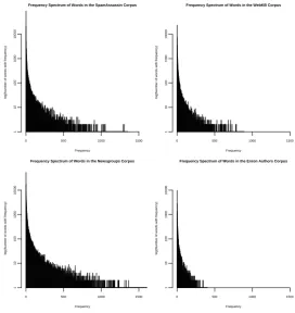
We present two quantifications of word reuse to support our conclusions. The first are frequency spectra for each of the four corpora, shown in Fig-ure 1. The two more problematic datasets appear in the top of the figure. To generate the charts, we pool all documents from all classes in a each prob-lem, and count the number of words that appear

once, twice, and so on. The x axis is the

num-ber of times a word occurs, and theyaxis the total

number of words which have that count.

The WebKB corpus has the large majority of words occurring very few times (the mass of the distribution is concentrated towards the left of the chart), while the SpamAssassin corpus is more rea-sonable and the Newsgroups corpus has by far the most words which occur with substantial fre-quency (this correlates perfectly with the relative performances of the classifiers on these datasets). For the Enron corpus, it is somewhat harder to tell, since its size means no words occur with substan-tial frequency.

We also consider the proportion of all word pairs in a corpus in which the first word is the same as

the second word. If a corpus has n• words total

with total countsn1...nv then the statistic is:

r= ₍_n 1

•(n•−1))/2 X

i

(ni(ni−1))/2. (14)

To measure differing tendencies to reuse words,

we calculate therstatistic once for each class, and

(7)

Newsgroups Enron Authors WebKB SpamAssassin Multinomial 85.66 ± 0.5 74.55 ± 1.34 85.69 ± 1.06 95.96 ± 0.5

DCM 85.03 ± 0.51 74.43 ± 1.34 82.69 ± 1.15 91.47 ± 0.7

Beta-Bin 91.65± 0.4∗+ _83.54_{± 1.14}∗+ _{84.81 ± 1.08} _{97.35 ± 0.4}∗

[image:7.595.83.512.73.146.2]

SVM 88.8 ± 0.45∗ _{80 ± 1.23}∗ _92.68_{± 0.79}∗ _97.65_{± 0.38}∗

Table 1: Performance of four classifiers on four tasks. Error is 95% interval for accuracy. Bold denotes

best performance on a task. ∗ _{denotes performance superior to multinomial which exceeds posterior}

uncertainty (i.e. observed performance outside 95% interval). +_{denotes the same for the SVM}

Frequency Spectrum of Words in the SpamAssassin Corpus

Frequency

log(Number of words with frequency)

1

10

100

1000

10000

0 500 1000 1500

Frequency Spectrum of Words in the WebKB Corpus

Frequency

1

10

100

1000

10000

0 500 1000 1500

Frequency Spectrum of Words in the Newsgroups Corpus

Frequency

1

10

100

1000

10000

0 500 1000 1500

Frequency Spectrum of Words in the Enron Authors Corpus

Frequency

1

10

100

1000

10000

0 500 1000 1500

Figure 1: Frequency spectra for the four datasets. yaxis is on a logarithmic scale

not look promising for the hierarchical model by either measure.

7 Conclusion

In this paper, we have advocated the use of a joint beta–binomial distribution for word counts in documents for the purposes of classification. We have shown that this model outperforms classifiers based upon both multinomial and Dirichlet Com-pound Multinomial distributions for word counts.

We have further made the case that, where cor-pora are sufficiently large as to warrant it, a gener-ative classifier employing a hierarchical sampling model outperforms a discriminative linear SVM. We attribute this to the capacity of the proposed model to capture aspects of word behaviour

be-yond a simpler model. However, in cases where the data contain many infrequent words and the tendency to reuse words is relatively low, default-ing to a linear classifier (either the multinomial for a generative classifier, or preferably the lin-ear SVM) increases performance relative to a more complex model, which cannot be fit with sufficient precision.

References

Allison, Ben and Louise Guthrie. 2008. Authorship at-tribution of e-mail: Comparing classifiers over a new corpus for evaluation. InProceedings of LREC’08. Brown, Lawrence D., Tony Cai, and Anirban

[image:7.595.159.432.212.501.2]

(8)

Newsgroups Enron Authors WebKB SpamAssassin

[image:8.595.93.504.73.104.2]

Meanr 0.0090 0.0083 0.0047 0.0037

Table 2: Meanrstatistic for the four problems

Church, K. and W. Gale. 1995. Poisson mixtures. Nat-ural Language Engineering, 1(2):163–190.

Dumais, Susan, John Platt, David Heckerman, and Mehran Sahami. 1998. Inductive learning algo-rithms and representations for text categorization. In

CIKM ’98, pages 148–155.

Elkan, Charles. 2006. Clustering documents with an exponential-family approximation of the dirich-let compound multinomial distribution. In Proceed-ings of the Twenty-Third International Conference on Machine Learning.

Eyheramendy, S., D. Lewis, and D. Madigan. 2003. The naive bayes model for text categorization. Arti-ficial Intelligence and Statistics.

Guthrie, Louise, Elbert Walker, and Joe Guthrie. 1994. Document classification by machine: theory and practice. InProceedings COLING ’94, pages 1059– 1063.

Jansche, Martin. 2003. Parametric models of linguistic count data. InACL ’03, pages 288–295.

Joachims, Thorsten. 1998. Text categorization with support vector machines: learning with many rele-vant features. In N´edellec, Claire and C´eline Rou-veirol, editors,Proceedings of ECML-98, 10th Euro-pean Conference on Machine Learning, pages 137– 142.

Joachims, Thorsten. 1999. Making large-scale svm learning practical. Advances in Kernel Methods -Support Vector Learning.

Katz, Slava M. 1996. Distribution of content words and phrases in text and language modelling. Nat. Lang. Eng., 2(1):15–59.

Klimt, Bryan and Yiming Yang. 2004. The enron cor-pus: A new dataset for email classification research. InProceedings of ECML 2004, pages 217–226. Lang, Ken. 1995. NewsWeeder: learning to filter

net-news. InProceedings of the 12th International Con-ference on Machine Learning, pages 331–339. Lasserre, Julia A., Christopher M. Bishop, and

Thomas P. Minka. 2006. Principled hybrids of gen-erative and discriminative models. In CVPR ’06: Proceedings of the 2006 IEEE Computer Society Conference on Computer Vision and Pattern Recog-nition, pages 87–94.

Lowe, S. 1999. The beta-binomial mixture model and its application to tdt tracking and detection. In Pro-ceedings of the DARPA Broadcast News Workshop.

Madsen, Rasmus E., David Kauchak, and Charles Elkan. 2005. Modeling word burstiness using the Dirichlet distribution. InICML ’05, pages 545–552. McCallum, A. and K. Nigam. 1998. A comparison

of event models for na¨ıve bayes text classification. InProceedings AAAI-98 Workshop on Learning for Text Categorization.

Minka, Tom. 2000. Estimating a dirichlet distribution. Technical report, Microsoft Research.

Rennie, Jason D. M. and Ryan Rifkin. 2001. Improv-ing multiclass text classification with the Support Vector Machine. Technical report, Massachusetts In-sititute of Technology, Artificial Intelligence Labora-tory.

Rennie, J., L. Shih, J. Teevan, and D. Karger. 2003. Tackling the poor assumptions of naive bayes text classifiers.