Predicting Discourse Connectives for Implicit Discourse Relation
Recognition
Zhi-Min Zhou and Yu Xu East China Normal University
Zheng-Yu Niu Toshiba China R&D Center [email protected]
Man Lan and Jian Su Institute for Infocomm Research [email protected]
Chew Lim Tan
National University of Singapore [email protected]
Abstract
Existing works indicate that the absence of explicit discourse connectives makes it difficult to recognize implicit discourse relations. In this paper we attempt to overcome this difficulty for implicit rela-tion recognirela-tion by automatically insert-ing discourse connectives between argu-ments with the use of a language model. Then we propose two algorithms to lever-age the information of these predicted connectives. One is to use these pre-dicted implicit connectives as additional features in a supervised model. The other is to perform implicit relation recognition based only on these predicted connectives. Results on Penn Discourse Treebank 2.0 show that predicted discourse connectives help implicit relation recognition and the first algorithm can achieve an absolute av-erage f-score improvement of 3% over a state of the art baseline system.
1 Introduction
Discourse relation analysis is to automatically identify discourse relations (e.g., explanation re-lation) that hold between arbitrary spans of text. This analysis may be a part of many natural lan-guage processing systems, e.g., text summariza-tion system, quessummariza-tion answering system. If there are discourse connectives between textual units to explicitly mark their relations, the recognition task on these texts is defined asexplicit discourse relation recognition. Otherwise it is defined as im-plicit discourse relation recognition.
Previous study indicates that the presence of discourse connectives between textual units can greatly help relation recognition. In Penn Dis-course Treebank (PDTB) corpus (Prasad et al., 2008), the most general senses, i.e., Comparison (Comp.), Contingency (Cont.), Temporal (Temp.) and Expansion (Exp.), can be disambiguated in explicit relations with more than 90% f-scores based only on the discourse connectives explicitly used to signal the relation (Pitler and Nenkova., 2009b).
However, for implicit relations, there are no connectives to explicitly mark the relations, which makes the recognition task quite difficult. Some of existing works attempt to perform relation recog-nition without hand-annotated corpora (Marcu and Echihabi, 2002), (Sporleder and Lascarides, 2008) and (Blair-Goldensohn, 2007). They use unambiguous patterns such as [Arg1, but Arg2] to create synthetic examples of implicit relations and then use [Arg1, Arg2] as an training example of an implicit relation. Another research line is to exploit various linguistically informed features under the framework of supervised models, (Pitler et al., 2009a) and (Lin et al., 2009), e.g., polarity features, semantic classes, tense, production rules of parse trees of arguments, etc.
possi-ble reason is that implicit connectives do not ex-ist in unannotated real texts. Another evidence of the importance of connectives for implicit re-lations is shown in PDTB annotation. The PDTB annotation consists of inserting a connective ex-pression that best conveys the inferred relation by the readers. Connectives inserted in this way to express inferred relations are calledimplicit con-nectives, which do not exist in real texts. These evidences inspire us to consider two interesting re-search questions:
(1) Can we automatically predict implicit connec-tives between arguments?
(2) How to use the predicted implicit connectives to build an automatic discourse relation analysis system?
In this paper we address these two questions as follows: (1) We insert appropriate discourse con-nectives between two textual units with the use of a language model. Here we train the language model on large amount of raw corpora without the use of any hand-annotated data. (2) Then we present two algorithms to use these predicted con-nectives for implicit relation recognition. One is to use these connectives as additional features in a supervised model. The other is to perform relation recognition based only on these connectives.
We performed evaluation of the two algorithms and a baseline system on PDTB 2.0 corpus. Ex-perimental results showed that using predicted discourse connectives as additional features can significantly improve the performance of implicit discourse relation recognition. Specifically, the first algorithm achieved an absolute average f-score improvement of 3% over a state of the art baseline system.
The rest of this paper is organized as follows. Section 2 describes the two algorithms for implicit discourse relation recognition. Section 3 presents experiments and results on PDTB data. Section 4 reviews related work. Section 5 concludes this work.
2 Our Algorithms for Implicit Discourse Relation Recognition
2.1 Prediction of implicit connectives
Explicit discourse relations are easily identifiable due to the presence of discourse connectives be-tween arguments. (Pitler and Nenkova., 2009b) showed that in PDTB corpus, the most general senses, i.e., Comparison (Comp.), Contingency (Cont.), Temporal (Temp.) and Expansion (Exp.), can be disambiguated in explicit relations with more than 90% f-scores based only on discourse connectives.
But for implicit relations, there are no connec-tives to explicitly mark the relations, which makes the recognition task quite difficult. PDTB data providesimplicit connectivesthat are inserted be-tween paragraph-internal adjacent sentence pairs not marked by any of explicit connectives. The availability of ground-truth implicit connectives makes it possible to evaluate the contribution of these connectives for implicit relation recognition. Our initial study on PDTB data show that the av-erage f-score for the most general 4 senses can reach 91.8% when we obtained the sense of each test example by mapping each ground truth im-plicit connective to its most frequent sense. We see that connective information is an important knowledge source for implicit relation recogni-tion. However these implicit connectives do not exist in real texts. In this paper we overcome this difficulty by inserting a connective between two arguments with the use of a language model.
Following the annotation scheme of PDTB, we assume that each implicit connective takes two ar-guments, denoted as Arg1 and Arg2. Typically, there are two possible positions for most of im-plicit connectives1, i.e., the position before Arg1 and the position between Arg1 and Arg2. Given a set of possible implicit connectives{ci}, we
gen-erate two synthetic sentences,ci+Arg1+Arg2 and
Arg1+ci+Arg2 for each ci, denoted as Sci,1 and Sci,2. Then we calculate the perplexity (an
intrin-sic score) of these sentences with the use of a lan-guage model, denoted asP P L(Sci,j). According
1For parallel connectives, e.g.,if. . .then. . . , the two
to the value ofP P L(Sci,j)(the lower the better),
we can rank these sentences and select the con-nectives in top N sentences as implicit
connec-tives for this argument pair. The language model may be trained on large amount of unannotated corpora that can be cheaply acquired, e.g., North American News corpus.
2.2 Using predicted implicit connectives as additional features
We predict implicit connectives on both training set and test set. Then we can use the predicted implicit connectives as additional features for su-pervised implicit relation recognition. Previous works exploited various linguistically informed features under the framework of supervised mod-els. In this paper, we include 9 types of features in our system due to their superior performance in previous studies, e.g., polarity features, seman-tic classes of verbs, contextual sense, modality, inquirer tags of words, first-last words of argu-ments, cross-argument word pairs, ever used in (Pitler et al., 2009a), production rules of parse trees of arguments used in (Lin et al., 2009), and intra-argument word pairs inspired by the work of (Saito et al., 2006).
Here we provide the details of the 9 features, shown as follows:
Verbs: Similar to the work in (Pitler et al., 2009a), the verb features consist of the number of pairs of verbs in Arg1 and Arg2 if they are from the same class based on their highest Levin verb class level (Dorr, 2001). In addition, the average length of verb phrase and the part of speech tags of main verb are also included as verb features.
Context:If the immediately preceding (or fol-lowing) relation is an explicit, its relation and sense are used as features. Moreover, we use an-other feature to indicate if Arg1 leads a paragraph. Polarity: We use the number of positive, negated positive, negative and neutral words in ar-guments and their cross product as features. For negated positives, we locate the negated words in text span and then define the closely behind posi-tive word as negated posiposi-tive.
Modality:We look for modal words including their various tenses or abbreviation forms in both arguments. Then we generate a feature to indicate
the presence or absence of modal words in both arguments and their cross product.
Inquirer Tags: Inquirer Tags extracted from General Inquirer lexicon (Stone et al., 1966) con-tains positive or negative classification of words. In fact, its fine-grained categories, such as Fall versus Rise, or Pleasure versus Pain, can indi-cate the relation between two words, especially for verbs. So we choose the presence or absence of 21 pair categories with complementary relation in Inquirer Tags as features. We also include their cross production as features.
FirstLastFirst3: We choose the first and last words of each argument as features, as well as the pair of first words, the pair of last words, and the first 3 words in each argument. In addition, we ap-ply Porter’s Stemmer (Porter, 1980) to each word before preparation of these features.
Production Rule: According to (Lin et al., 2009), we extract all the possible production rules from arguments, and check whether the rules ap-pear in Arg1, Arg2 and both arguments. We re-move the rules occurring less than 5 times in train-ing data.
Cross-argument Word Pairs:We perform the Porter’s stemming (Porter, 1980), and then group all words from Arg1 and Arg2 into two setsW1 andW2respectively. Then we generate any possi-ble word pair (wi,wj) (wi ∈ W1,wj ∈W2). We
remove the word pairs with less than 5 times. Intra-argument Word Pairs: Let
Q1 = (q1, q2, . . . , qn) be the word
se-quence of Arg1. The intra-argument word pairs for Arg1 is defined as W P1 =
((q1, q2),(q1, q3), . . . ,(q1, qn),(q2, q3), . . . ,
(qn−1, qn)). We extract all the intra-argument
word pairs from Arg1 and Arg2 and remove word pairs appearing less than 5 times in training data.
2.3 Relation recognition based only on predicted implicit connectives
of connectives are unambiguous and it is possible to obtain high performance in prediction of dis-course sense due to the simple mapping relation between connectives and senses. Given two ex-amples:
(E1) She paid less on her dress,butit is very nice. (E2) We have to harry up becausethe raining is getting heavier and heavier.
The two connectives, i.e.,butin E1 and because in E2, convey Comparison and Contingency sense respectively. In most cases, we can easily recog-nize the relation sense by the appearance of dis-course connective since it can be interpreted in only one way. That means, the ambiguity of the mapping between sense and connective is quite few.
We count the frequency of sense tags for each possible connective on PDTB training data for im-plicit relation. Then we build a sense recognition model by simply mapping each connective to its most frequent sense. Here we do not perform con-nective prediction on training data. During test-ing, we use the language model to insert implicit connectives into each test argument pair. Then we perform relation recognition by mapping each im-plicit connective to its most frequent sense.
3 Experiments and Results 3.1 Experiments
3.1.1 Data sets
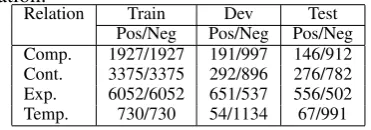
In this work we used the PDTB 2.0 corpus for evaluation of our algorithms. Following the work of (Pitler et al., 2009a), we used sections 2-20 as training set, sections 21-22 as test set, and sec-tions 0-1 as development set for parameter opti-mization. For comparison with the work of (Pitler et al., 2009a), we ran four binary classification tasks to identify each of the main relations (Cont., Comp., Exp., and Temp.) from the rest. For each relation, we used equal numbers of positive and negative examples as training data2. The negative examples were chosen at random from sections 2-20. We used all the instances in sections 21 and 22 as test set, so the test set is representative of 2Here the numbers of training and test instances for
Ex-pansion relation are different from those in (Pitler et al., 2009a). The reason is that we do not include instances of EntRel as positive examples.
[image:4.595.316.502.166.231.2]the natural distribution. The numbers of positive and negative instances for each sense in different data sets are listed in Table 1.
Table 1: Statistics of positive and negative sam-ples in training, development and test sets for each relation.
Relation Train Dev Test
Pos/Neg Pos/Neg Pos/Neg Comp. 1927/1927 191/997 146/912 Cont. 3375/3375 292/896 276/782 Exp. 6052/6052 651/537 556/502 Temp. 730/730 54/1134 67/991
In this work we used LibSVM toolkit to con-struct four linear SVM models for a baseline sys-tem and the syssys-tem in Section 2.2.
3.1.2 A baseline system
We first built a baseline system, which used 9 types of features listed in Section 2.2.
We tuned the numbers of firstLastFirst3, cross-argument word pair, intra-cross-argument word pair on development set. Finally we set the frequency threshold at 3, 5 and 5 respectively.
3.1.3 Prediction of implicit connectives To predict implicit connectives, we adopt the following two steps:(1) train a language model; (2) select top N implicit connectives.
Step 1:We used SRILM toolkit to train the lan-guage models on three benchmark news corpora, i.e., New York part in the BLLIP North Ameri-can News, Xin and Ltw parts of English Gigaword (4th Edition). We also tried different values for
nin n-gram model. The parameters were tuned
on the development set to optimize the accuracy of prediction. In this work we chose 3-gram lan-guage model trained on NY corpus.
Step 2:We combined each instance’s Arg1 and Arg2 with connectives extract from PDTB2 (100 in all). There are two types of connectives, sin-gle connective (e.g. becauseandbut) and paral-lel connective (such as “not only. . . , but also”). Since discourse connectives may appear not only ahead of the Arg1, but also between Arg1 and Arg2, we considered this case. Given a set of pos-sible implicit connectives{ci}, for single
parallel connective, we constructed one synthetic sentence likeci1+Arg1+ci2+Arg2.
As a result, we can get 198 synthetic sentences for each argument pair. Then we converted all words to lower cases and used the language model trained in the above step to calculate perplexity on sentence level. The perplexity scores were ranked from low to high. For example, we got the perplexity (ppl) for two sentences as follows: (1) but this is an old story, we’re talking about years ago before anyone heard of asbestos having any questionable properties.
ppl= 652.837
(2) this is an old story, but we’re talking about years ago before anyone heard of asbestos having any questionable properties.
ppl= 583.514
We considered the combination of connectives and their position as final features like mid but, first but, where the features are binary, that is, the presence and absence of the specific connective.
According to the value of P P L(Sci,j) (the
lower the better), we selected the connectives in top N sentences as implicit connectives for this
argument pair. In order to get the optimalNvalue,
we tried various values ofN on development set and selected the minimum value ofN so that the
ground-truth connectives appeared in topN
con-nectives. The finalN value is set to 60 based on
the trade-off between performance and efficiency.
3.1.4 Using predicted connectives as additional features
This system combines the predicted implicit connectives as additional features and the 9 types of features in an supervised framework. The 9 types of features are listed as shown in Section 2.2 and tuned on development set.
We combined predicted connectives with the best subset features from the development data set with respect to f-score. In our experiment of se-lecting best subset features, single features rather than the combination of several features achieved much higher scores. So we combine single fea-tures with predicted connectives as final feafea-tures.
3.1.5 Using only predicted connectives for implicit relation recognition
We built two variants for the algorithm in Sec-tion 2.3. One is to use the data for explicit re-lations in PDTB sections 2-20 as training data. The other is to use the data for implicit relations in PDTB sections 2-20 as training data. Given training data, we obtained the most frequent sense for each connective appearing in the training data. Then given test data, we recognized the sense of each argument pair by mapping each predicted connective to its most frequent sense. In this work we conducted another experiment to see the upper-bound performance of this algorithm. Here we performed recognition based on ground-truth implicit connectives and used the data for implicit relations as training data.
3.2 Results
3.2.1 Result of baseline system
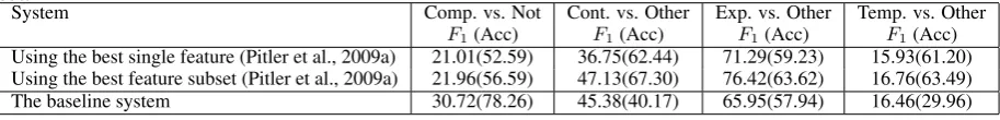
Table 2 summarizes the best performance achieved by the baseline system in compari-son with previous state-of-the-art performance achieved in (Pitler et al., 2009a). The first two lines in the table show their best results using sin-gle feature and using combined feature subset. It indicates that the performance of using combined feature subset is higher than that using single fea-ture alone.
From this table, we can find that our base-line system has a comparable result on Contin-gency and Temporal. On Comparison, our system achieved a better performance around 9% f-score higher than their best result. However, for Expan-sion, they expanded both training and testing sets by including EntRel relation as positive examples, which makes it impossible to perform direct com-parison. Generally, our baseline system is reason-able and thus the consequent experiments on it are reliable.
Table 2: Performance comparison of the baseline system with the system of (Pitler et al., 2009a) on test set.
System Comp. vs. Not Cont. vs. Other Exp. vs. Other Temp. vs. Other
F1(Acc) F1(Acc) F1(Acc) F1(Acc)
Using the best single feature (Pitler et al., 2009a) 21.01(52.59) 36.75(62.44) 71.29(59.23) 15.93(61.20) Using the best feature subset (Pitler et al., 2009a) 21.96(56.59) 47.13(67.30) 76.42(63.62) 16.76(63.49)
The baseline system 30.72(78.26) 45.38(40.17) 65.95(57.94) 16.46(29.96)
[image:6.595.74.296.260.521.2]the first algorithm using predicted connectives as additional features.
Table 3: Performance comparison of the algo-rithm in Section 2.2 with the baseline system on test set.
Rela- Features Baseline Baseline+LM
tion F1(Acc) F1(Acc)
Comp. Production Rule 30.72(78.26) 31.08(68.15) Context 24.66(42.25) 27.64(53.97) InquirerTags 23.31(73.25) 27.87(55.48) Polarity 21.11(40.64) 23.64(52.36) Modality 17.25(80.06) 26.17(55.20) Verbs 25.00(53.50) 31.79(58.22) Cont. Prodcution Rule 45.38(40.17) 47.16(48.96) Context 37.61(44.70) 34.74(48.87) Polarity 35.57(50.00) 43.33(33.74) InquirerTags 38.04(41.49) 42.22(36.11) Modality 32.18(66.54) 35.26(55.58) Verbs 40.44(54.06) 42.04(32.23) Exp. Context 48.34(54.54) 68.32(53.02) FirstLastFirst3 65.95(57.94) 68.94(53.59) InquirerTags 61.29(52.84) 68.49(53.21) Modality 64.36(56.14) 68.9(52.55) Polarity 49.95(50.38) 68.62(53.40) Verbs 52.95(53.31) 70.11(54.54) Temp. Context 13.52(64.93) 16.99(79.68) FirstLastFirst3 15.75(66.64) 19.70(64.56) InquirerTags 8.51(83.74) 19.20(56.24) Modality 16.46(29.96) 19.97(54.54) Polarity 16.29(51.42) 20.30(55.48) Verbs 13.88(54.25) 13.53(61.34)
From this table, we found that this additional feature obtained from language model showed significant improvements in almost four relations. Specifically, the top two improvements are on Ex-pansion and Temporal relations, which improved 4.16% and 3.84% in f-score respectively. Al-though on Comparison relation there is only a slight improvement (+1.07%), our two best sys-tems both got around 10% improvements of f-score over a state-of-the-art system in (Pitler et al., 2009a). As a whole, the first algorithm achieved 3% improvement of f-score over a state of the art baseline system. All these results indicate that predicted implicit connectives can help improve
the performance.
3.2.3 Result of algorithm 2: using only predicted connectives for implicit relation recognition
Table 4 summarizes the best performance achieved by the second algorithm in comparison with the baseline system on test set.
The experiment showed that the baseline sys-tem using just gold-truth implicit connectives can achieve an f-score of 91.8% for implicit relation recognition. It once again proved that implicit connectives make significant contributions for im-plicit relation recognition. This also encourages our future work on finding the most suitable con-nectives for implicit relation recognition.
From this table, we found that, using only pre-dicted implicit connectives achieved an compara-ble performance to (Pitler et al., 2009a), although it was still a bit lower than our best baseline. But we should bear in mind that this algorithm only uses 4 features for implicit relation recognition and these 4 features are easy computable and fast run, which makes the system more practical in ap-plication. Furthermore, compared with other al-gorithms which require hand-annotated data for training, the performance of this second algorithm is acceptable if we take into account that no la-beled data is used for model training.
3.3 Analysis
Table 4: Performance comparison of the algorithm in Section 2.3 with the baseline system on test set.
System Comp. vs. Other Cont. vs. Other Exp. vs. Other Temp. vs. Other
F1(Acc) F1(Acc) F1(Acc) F1(Acc)
The baseline system 30.72(78.26) 45.38(40.17) 65.95(57.94) 16.46(29.96)
Our algorithm with training data for explicit relation 26.02(52.17) 35.72(51.70) 64.94(53.97) 13.76(41.97) Our algorithm with training data for implicit relation 24.55(63.99) 16.26(70.79) 60.70(53.50) 14.75(70.51) Sense recognition using gold-truth implicit connectives 94.08(98.30) 98.19(99.05) 97.79(97.64) 77.04(97.07)
used different selection of instances for Expan-sion sense3, we cannot make a direct compari-son. However, we achieve the best f-score around 70%, which provide 5% improvements over our baseline system. On the other hand, the second proposed algorithm using only predicted connec-tives still achieves promising results for each rela-tion. Specifically, the model for the Comparison relation achieves an f-score of 26.02% (5% over the previous work in (Pitler et al., 2009a)). Fur-thermore, the models for Contingency and Tem-poral relation achieve 35.72% and 13.76% f-score respectively, which are comparable to the previ-ous work in (Pitler et al., 2009a). The model for Expansion relation obtains an f-score of 64.95%, which is only 1% less than our baseline system which consists of ten thousands of features.
4 Related Work
Existing works on automatic recognition of dis-course relations can be grouped into two cat-egories according to whether they used hand-annotated corpora.
One research line is to perform relation recog-nition without hand-annotated corpora.
(Marcu and Echihabi, 2002) used a pattern-based approach to extract instances of discourse relations such as Contrast and Elaboration from unlabeled corpora. Then they used word-pairs be-tween two arguments as features for building clas-sification models and tested their model on artifi-cial data for implicit relations.
There are other efforts that attempt to extend the work of (Marcu and Echihabi, 2002). (Saito et al., 2006) followed the method of (Marcu and Echi-habi, 2002) and conducted experiments with com-bination of cross-argument word pairs and phrasal
3They expanded the Expansion data set by adding
ran-domly selected EntRel instances by 50%, which is consid-ered to significantly change data distribution.
patterns as features to recognize implicit relations between adjacent sentences in a Japanese corpus. They showed that phrasal patterns extracted from a text span pair provide useful evidence in the re-lation classification. (Sporleder and Lascarides, 2008) discovered that Marcu and Echihabi’s mod-els do not perform as well on implicit relations as one might expect from the test accuracies on syn-thetic data. (Blair-Goldensohn, 2007) extended the work of (Marcu and Echihabi, 2002) by re-fining the training and classification process using parameter optimization, topic segmentation and syntactic parsing.
(Lapata and Lascarides, 2004) dealt with tem-poral links between main and subordinate clauses by inferring the temporal markers linking them. They extracted clause pairs with explicit temporal markers from BLLIP corpus as training data.
Another research line is to use human-annotated corpora as training data, e.g., the RST Bank (Carlson et al., 2001) used by (Soricut and Marcu, 2003), adhoc annotations used by (?), (Baldridge and Lascarides, 2005), and the Graph-Bank (Wolf et al., 2005) used by (Wellner et al., 2006).
In comparison with existing works, we investi-gated a new knowledge source, implicit connec-tives, for implicit relation recognition. Moreover, our two models can exploit both labeled and labeled data by training a language model on un-labeled data and then using this language model to generate implicit connectives for recognition models trained on labeled data.
5 Conclusions
In this paper we use a language model to auto-matically generate implicit connectives and then present two methods to use these connectives for recognition of implicit relations. One method is to use these predicted implicit connectives as addi-tional features in a supervised model and the other is to perform implicit relation recognition based only on these predicted connectives. Results on Penn Discourse Treebank 2.0 show that predicted discourse connectives help implicit relation recog-nition and the first algorithm achieves an absolute average f-score improvement of 3% over a state of the art baseline system.
Acknowledgments
This work is supported by grants from Na-tional Natural Science Foundation of China (No.60903093), Shanghai Pujiang Talent Program (No.09PJ1404500) and Doctoral Fund of Ministry of Education of China (No.20090076120029).
References
J. Baldridge and A. Lascarides. 2005. Probabilistic head-driven parsing for discourse structure. Pro-ceedings of the Ninth Conference on Computational Natural Language Learning.
L. Carlson, D. Marcu, and Ma. E. Okurowski. 2001. Building a discourse-tagged corpus in the frame-work of rhetorical structure theory. Proceedings of the Second SIG dial Workshop on Discourse and Di-alogue.
B. Dorr. LCS Verb Database. Technical Report Online Software Database, University of Maryland, Col-lege Park, MD,2001.
R. Girju. 2003. Automatic detection of causal rela-tions for question answering. In ACL 2003 Work-shops.
S. Blair-Goldensohn. 2007. Long-Answer Ques-tion Answering and Rhetorical-Semantic RelaQues-tions. Ph.D. thesis, Columbia Unviersity.
M. Lapata and A. Lascarides. 2004. Inferring Sentence-internal Temporal Relations. Proceedings of the North American Chapter of the Assocation of Computational Linguistics.
Z.H. Lin, M.Y. Kan and H.T. Ng. 2009. Recognizing Implicit Discourse Relations in the Penn Discourse Treebank. Proceedings of the 2009 Conference on EMNLP.
D. Marcu and A. Echihabi. 2002. An Unsupervised Approach to Recognizing Discourse Relations. Pro-ceedings of the 40th ACL.
E. Pitler, A. Louis, A. Nenkova. 2009. Automatic sense prediction for implicit discourse relations in text. Proceedings of the 47th ACL.
E. Pitler and A. Nenkova. 2009. Using Syntax to Dis-ambiguate Explicit Discourse Connectives in Text. Proceedings of the ACL-IJCNLP 2009 Conference Short Papers.
M. Porter. 1980. An algorithm for suffix stripping. In Program, vol. 14, no. 3, pp.130-137.
R. Prasad, N. Dinesh, A. Lee, E. Miltsakaki, L. Robaldo, A. Joshi, B. Webber. 2008.The Penn Dis-course TreeBank 2.0. Proceedings of LREC’08.
M. Saito, K.Yamamoto, S.Sekine. 2006. Using Phrasal Patterns to Identify Discourse Relations. Proceeding of the HLTCNA Chapter of the ACL.
R. Soricut and D. Marcu. Sentence Level Discourse Parsing using Syntactic and Lexical Information. Proceedings of HLT/NAACL 2003.
C. Sporleder and A. Lascarides. 2008.Using automat-ically labelled examples to classify rhetorical rela-tions: an assessment. Natural Language Engineer-ing, Volume 14, Issue 03.
P.J. Stone, J. Kirsh, and Cambridge Computer Asso-ciates. 1966. The General Inquirer: A Computer Approach to Content Analysis. MIT Press.
B. Wellner , J. Pustejovsky, C. H. R. S., A. Rumshisky. 2006. Classification of discourse coherence rela-tions: An exploratory study using multiple knowl-edge sources. Proceedings of the 7th SIGDIAL Workshop on Discourse and Dialogue.