Word Graphs for Statistical Machine Translation
Richard ZensandHermann Ney Chair of Computer Science VI
RWTH Aachen University
{zens,ney}@cs.rwth-aachen.de
Abstract
Word graphs have various applications in the field of machine translation. Therefore it is important for machine translation sys-tems to produce compact word graphs of high quality. We will describe the gen-eration of word graphs for state of the art phrase-based statistical machine trans-lation. We will use these word graph to provide an analysis of the search pro-cess. We will evaluate the quality of the word graphs using the well-known graph word error rate. Additionally, we intro-duce the two novel graph-to-string crite-ria: the position-independent graph word error rate and the graph BLEU score. Experimental results are presented for two Chinese–English tasks: the small IWSLT task and the NIST large data track task. For both tasks, we achieve significant re-ductions of the graph error rate already with compact word graphs.
1 Introduction
A statistical machine translation system usually pro-duces the single-best translation hypotheses for a source sentence. For some applications, we are also interested in alternative translations. The simplest way to represent these alternatives is a list with the
N-best translation candidates. These N-best lists
have one major disadvantage: the high redundancy. The translation alternatives may differ only by a sin-gle word, but still both are listed completely.
Usu-ally, the size of theN-best list is in the range of a few
hundred up to a few thousand candidate translations
per source sentence. If we want to use largerN-best
lists the processing time gets very soon infeasible. Word graphs are a much more compact represen-tation that avoid these redundancies as much as pos-sible. The number of alternatives in a word graph is
usually an order of magnitude larger than in anN
-best list. The graph representation avoids the
com-binatorial explosion that make largeN-best lists
in-feasible.
Word graphs are an important data structure with various applications:
• Word Filter.
The word graph is used as a compact repre-sentation of a large number of sentences. The score information is not contained.
• Rescoring.
We can use word graphs for rescoring with more sophisticated models, e.g. higher-order language models.
• Discriminative Training.
The training of the model scaling factors as de-scribed in (Och and Ney, 2002) was done on
N-best lists. Using word graphs instead could
further improve the results. Also, the phrase translation probabilities could be trained dis-crimatively, rather than only the scaling factors.
• Confidence Measures.
• Interactive Machine Translation.
Some interactive machine translation systems make use of word graphs, e.g. (Och et al., 2003).
State Of The Art.Although there are these many applications, there are only few publications directly devoted to word graphs. The only publication, we are aware of, is (Ueffing et al., 2002). The short-comings of (Ueffing et al., 2002) are:
• They use single-word based models only.
Cur-rent state of the art statistical machine transla-tion systems are phrase-based.
• Their graph pruning method is suboptimal as it
considers only partial scores and not full path scores.
• The N-best list extraction does not eliminate
duplicates, i.e. different paths that represent the same translation candidate.
• The rest cost estimation is not efficient. It has
an exponential worst-case time complexity. We will describe an algorithm with linear worst-case complexity.
Apart from (Ueffing et al., 2002), publications on weighted finite state transducer approaches to ma-chine translation, e.g. (Bangalore and Riccardi, 2001; Kumar and Byrne, 2003), deal with word graphs. But to our knowledge, there are no publica-tions that give a detailed analysis and evaluation of the quality of word graphs for machine translation.
We will fill this gap and give a systematic descrip-tion and an assessment of the quality of word graphs for phrase-based machine translation. We will show that even for hard tasks with very large vocabulary and long sentences the graph error rate drops signif-icantly.
The remaining part is structured as follows: first we will give a brief description of the translation sys-tem in Section 2. In Section 3, we will give a def-inition of word graphs and describe the generation.
We will also present efficient pruning and N-best
list extraction techniques. In Section 4, we will de-scribe evaluation criteria for word graphs. We will use the graph word error rate, which is well known from speech recognition. Additionally, we introduce the novel position-independent word graph error rate
and the graph BLEU score. These are generaliza-tions of the commonly used string-to-string evalua-tion criteria in machine translaevalua-tion. We will present experimental results in Section 5 for two Chinese– English tasks: the first one, the IWSLT task, is in the domain of basic travel expression found in phrase-books. The vocabulary is limited and the sentences are short. The second task is the NIST Chinese– English large data track task. Here, the domain is news and therefore the vocabulary is very large and the sentences are with an average of 30 words quite long.
2 Translation System
In this section, we give a brief description of the translation system. We use a phrase-based transla-tion approach as described in (Zens and Ney, 2004).
The posterior probabilityP r(eI
1|f1J)is modeled
di-rectly using a weighted log-linear combination of a trigram language model and various translation models: a phrase translation model and a word-based lexicon model. These translation models are
used for both directions: p(f|e) andp(e|f).
Addi-tionally, we use a word penalty and a phrase penalty. With the exception of the language model, all mod-els can be considered as within-phrase modmod-els as they depend only on a single phrase pair, but not on the context outside of the phrase. The model scaling factors are optimized with respect to some evalua-tion criterion (Och, 2003).
We extended the monotone search algorithm from (Zens and Ney, 2004) such that reorderings are pos-sible. In our case, we assume that local reorder-ings are sufficient. Within a certain window, all possible permutations of the source positions are al-lowed. These permutations are represented as a re-ordering graph, similar to (Zens et al., 2002). Once we have this reordering graph, we perform a mono-tone phrase-based translation of this graph. More details of this reordering approach are described in (Kanthak et al., 2005).
3 Word Graphs
3.1 Definition
A word graph is a directed acyclic graphG= (V, E)
with one designated root noden0 ∈ V. The edges
are labeled with words and optionally with scores.
nto noden0 with word labelw. Each path through
the word graph represents a translation candidate. If the word graph contains scores, we accumulate the edge scores along a path to get the sentence or string score.
The score information the word graph has to con-tain depends on the application.
If we want to use the word graph as a word fil-ter, we do not need any score information at all. If
we want to extract the single- orN-best hypotheses,
we have to retain the string or sentence score infor-mation. The information about the hidden variables of the search, e.g. the phrase segmentation, is not needed for this purpose. For discriminative training of the phrase translation probabilities, we need all the information, even about the hidden variables.
3.2 Generation
In this section, we analyze the search process in de-tail. Later, in Section 5, we will show the (experi-mental) complexity of each step. We start with the source language sentence that is represented as a lin-ear graph. Then, we introduce reorderings into this graph as described in (Kanthak et al., 2005). The type of reordering should depend on the language pair. In our case, we assume that only local reorder-ings are required. Within a certain window, all pos-sible reorderings of the source positions are allowed. These permutations are represented as a reordering graph, similar to (Knight and Al-Onaizan, 1998) and (Zens et al., 2002).
Once we have this reordering graph, we perform a monotone phrase-based translation of this graph. This translation process consists of the following steps that will be described afterward:
1. segment into phrase
2. translate the individual phrases 3. split the phrases into words 4. apply the language model
Now, we will describe each step. The first step is the segmentation into phrases. This can be imag-ined as introducing “short-cuts” into the graph. The phrase segmentation does not affect the number of nodes, because only additional edges are added to the graph.
In the segmented graph, each edge represents a source phrase. Now, we replace each edge with one
edge for each possible phrase translation. The edge scores are the combination of the different transla-tion probabilities, namely the within-phrase models mentioned in Section 2. Again, this step does not increase the number of nodes, but only the number of edges.
So far, the edge labels of our graph are phrases. In the final word graph, we want to have words as edge labels. Therefore, we replace each edge representing a multi-word target phrase with a sequence of edges that represent the target word sequence. Obviously, edges representing a single-word phrase do not have to be changed.
As we will show in the results section, the word graphs up to this point are rather compact. The score information in the word graph so far consists of the reordering model scores and the phrase trans-lation model scores. To obtain the sentence posterior
probabilityp(eI
1|f1J), we apply the target language
model. To do this, we have to separate paths accord-ing to the language model history. This increases the word graph size by an order of magnitude.
Finally, we have generated a word graph with full sentence scores. Note that the word graph may con-tain a word sequence multiple times with different hidden variables. For instance, two different seg-mentations into source phrases may result in the same target sentence translation.
The described steps can be implemented using weighted finite state transducer, similar to (Kumar and Byrne, 2003).
3.3 Pruning
To adjust the size of the word graph to the desired density, we can reduce the word graph size using forward-backward pruning, which is well-known in the speech recognition community, e.g. see (Mangu et al., 2000). This pruning method guarantees that the good strings (with respect to the model scores) remain in the word graph, whereas the bad ones are removed. The important point is that we compare the full path scores and not only partial scores as, for instance, in the beam pruning method in (Ueffing et al., 2002).
The forward probabilities F(n) and backward
following recursive equations:
F(n) = X
(n0,n,w)∈E
F(n0 )·p(n0
, n, w)
B(n) = X
(n,n0,w)∈E
B(n0
)·p(n, n0
, w)
The forward probability of the root node and the backward probabilities of the final nodes are initial-ized with one. Using a topological sorting of the nodes, the forward and backward probabilities can be computed with linear time complexity. The
pos-terior probability q(n, n0, w) of an edge is defined
as:
q(n, n0
, w) = F(n)·p(n, n
0, w)·B(n0)
B(n0)
The posterior probability of an edge is identical to the sum over the probabilities of all full paths that contain this edge. Note that the backward
probabil-ity of the root node B(n0) is identical to the sum
over all sentence probabilities in the word graph.
Let q∗ denoted the maximum posterior probability
of all edges and letτ be a pruning threshold, then
we prune an edge(n, n0, w
)if:
q(n, n0
, w) < q∗
·τ
3.4 N-Best List Extraction
In this section, we describe the extraction of theN
-best translation candidates from a word graph. (Ueffing et al., 2002) and (Mohri and Riley, 2002) both present an algorithm based on the same idea: use a modified A* algorithm with an optimal rest cost estimation. As rest cost estimation, the negated logarithm of the backward probabilities is used. The algorithm in (Ueffing et al., 2002) has two disadvan-tages: it does not care about duplicates and the rest cost computation is suboptimal as the described al-gorithm has an exponential worst-case complexity. As mentioned in the previous section, the backward probabilities can be computed in linear time.
In (Mohri and Riley, 2002) the word graph is rep-resented as a weighted finite state automaton. The word graph is first determinized, i.e. the nondeter-ministic automaton is transformed in an equivalent deterministic automaton. This process removes the duplicates from the word graph. Out of this
deter-minized word graph, theN best candidates are
ex-tracted. In (Mohri and Riley, 2002),²-transitions are
ignored, i.e. transitions that do not produce a word.
These²-transitions usually occur in the backing-off
case of language models. The²-transitions have to
be removed before using the algorithm of (Mohri
and Riley, 2002). In the presence of ²-transitions,
two path representing the same string are considered
equal only if the²-transitions are identical as well.
4 Evaluation Criteria
4.1 String-To-String Criteria
To evaluate the single-best translation hypotheses, we use the following string-to-string criteria: word error rate (WER), position-independent word error rate (PER) and the BLEU score. More details on these standard criteria can be found for instance in (Och, 2003).
4.2 Graph-To-String Criteria
To evaluate the quality of the word graphs, we generalize the string-to-string criteria to work on word graphs. We will use the well-known graph word error rate (GWER), see also (Ueffing et al., 2002). Additionally, we introduce two novel graph-to-string criteria, namely the position-independent graph word error rate (GPER) and the graph BLEU score (GBLEU). The idea of these graph-to-string criteria is to choose a sequence from the word graph and compute the corresponding string-to-string cri-terion for this specific sequence. The choice of the sequence is such that the criterion is the optimum over all possible sequences in the word graph, i.e. the minimum for GWER/GPER and the maximum for GBLEU.
The GWER is a generalization of the word
er-ror rate. It is a lower bound for the WER. It can be computed using a dynamic programming algorithm which is quite similar to the usual edit distance com-putation. Visiting the nodes of the word graph in topological order helps to avoid repeated computa-tions.
The GPER is a generalization of the
position-independent word error rate. It is a lower bound for the PER. The computation is not as straightforward as for the GWER.
we will first describe an alternative computation for the string-to-string PER and then use this idea for the graph-to-string PER.
Now, we want to compute the number of position-independent errors for two strings. As the word or-der of the strings does not matter, we represent them
as multisets1 AandB. To do this, it is sufficient to
know how many words are in A but not inB, i.e.
a:=|A−B|, and how many words are inBbut not
inA, i.e.b:=|B−A|. The number of substitutions,
insertions and deletions are then:
sub = min{a, b} ins = a−sub
del = b−sub
error = sub+ins+del
= a+b−min{a, b}
= max{a, b}
It is obvious that there are either no insertions or no deletions. The PER is then computed as the num-ber of errors divided by the length of the reference string.
Now, back to the graph-to-string PER computa-tion. The information we need at each node of the word graph are the following: the remaining multi-set of words of the reference string that are not yet
produced. We denote this multisetC. The
cardinal-ity of this multiset will become the value a in the
preceding notation. In addition to this multiset, we also need to count the number of words that we have produced on the way to this node but which are not in the reference string. The identity of these words is not important, we simply have to count them. This
count will become the valuebin the preceding
nota-tion.
If we make a transition to a successor node along
an edge labeledw, we remove that wordwfrom the
set of remaining reference wordsC or, if the word
wis not in this set, we increase the count of words
that are in the hypothesis but not in the reference. To compute the number of errors on a graph, we
use the auxiliary quantity Q(n, C), which is the
count of the produced words that are not in the refer-ence. We use the following dynamic programming recursion equations:
1A multiset is a set that may contain elements multiple times.
Q(n0, C0) = 0
Q(n, C) = min
n0,w:(n0,n,w)∈E
n Q(n0
, C∪ {w}),
Q(n0
, C) + 1o
Here,n0 denote the root node of the word graph,
C0 denotes the multiset representation of the
refer-ence string. As already mentioned in Section 3.1,
(n0, n, w
)denotes an edge from node n0 to noden
with word labelw.
In the implementation, we use a bit vector to
rep-resent the setC for efficiency reasons. Note that in
the worst-case the size of the Q-table is
exponen-tial in the length of the reference string. However, in practice we found that in most cases the computation is quite fast.
The GBLEU score is a generalization of the BLEU score. It is an upper bound for the BLEU score. The computation is similar to the GPER com-putation. We traverse the word graph in topologi-cal order and store the following information: the
counts of the matchingn-grams and the length of the
hypothesis, i.e. the depth in the word graph.
Addi-tionally, we need the multiset of referencen-grams
that are not yet produced.
To compute the BLEU score, the n-gram counts
are collected over the whole test set. This results in a combinatorial problem for the computation of the GBLEU score. We process the test set sentence-wise
and accumulate then-gram counts. After each
sen-tence, we take a greedy decision and choose then
-gram counts that, if combined with the accumulated
n-gram counts, result is the largest BLEU score.
This gives a conservative approximation of the true GBLEU score.
4.3 Word Graph Size
To measure the word graph size we use the word graph density, which we define as the number of edges in the graph divided by the source sentence length.
5 Experimental Results
5.1 Tasks
Table 1: IWSLT Chinese–English Task: corpus statistics of the bilingual training data.
Chinese English
Train Sentences 20 000
Running Words 182 904 160 523
Vocabulary 7 643 6 982
Test Sentences 506
Running Words 3 515 3 595
[image:6.612.316.534.59.213.2]avg. SentLen 6.9 7.1
Table 2: NIST Chinese English task: corpus statis-tics of the bilingual training data.
Chinese English
Train Sentences 3.2M
Running Words 51.4M 55.5M
Vocabulary 80 010 170 758
Lexicon Entries 81 968
Test Sentences 878
Running Words 26 431 23 694
avg. SentLen 30.1 27.0
IWSLT Chinese–English Task. The first task is the Chinese–English supplied data track task of the International Workshop on Spoken Language Trans-lation (IWSLT 2004) (Akiba et al., 2004). The do-main is travel expressions from phrase-books. This is a small task with a clean training and test corpus. The vocabulary is limited and the sentences are rel-atively short. The corpus statistics are shown in Ta-ble 1. The Chinese part of this corpus is already segmented into words.
NIST Chinese–English Task. The second task is the NIST Chinese–English large data track task. For this task, there are many bilingual corpora avail-able. The domain is news, the vocabulary is very large and the sentences have an average length of 30 words. We train our statistical models on various corpora provided by LDC. The Chinese part is seg-mented using the LDC segmentation tool. After the preprocessing, our training corpus consists of about three million sentences with somewhat more than 50 million running words. The corpus statistics of the preprocessed training corpus are shown in Table 2. We use the NIST 2002 evaluation data as test set.
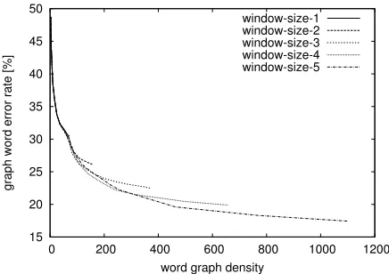
15 20 25 30 35 40 45 50
0 200 400 600 800 1000 1200
graph word error rate [%]
word graph density window-size-1 window-size-2 window-size-3 window-size-4 window-size-5
Figure 1: IWSLT Chinese–English: Graph error rate as a function of the word graph density for different window sizes.
5.2 Search Space Analysis
In Table 3, we show the search space statistics of the IWSLT task for different reordering window sizes. Each line shows the resulting graph densities after the corresponding step in our search as described in Section 3.2. Our search process starts with the re-ordering graph. The segmentation into phrases in-creases the graph densities by a factor of two. Doing the phrase translation results in an increase of the densities by a factor of twenty. Unsegmenting the phrases, i.e. replacing the phrase edges with a se-quence of word edges doubles the graph sizes. Ap-plying the language model results in a significant in-crease of the word graphs.
Another interesting aspect is that increasing the window size by one roughly doubles the search space.
5.3 Word Graph Error Rates
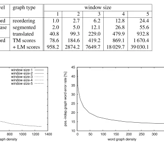
[image:6.612.77.292.92.190.2]Table 3: IWSLT Chinese–English: Word graph densities for different window sizes and different stages of the search process.
language level graph type window size
1 2 3 4 5
source word reordering 1.0 2.7 6.2 12.8 24.4
phrase segmented 2.0 5.0 12.1 26.8 55.6
target translated 40.8 99.3 229.0 479.9 932.8
word TM scores 78.6 184.6 419.2 869.1 1 670.4
+ LM scores 958.2 2874.2 7649.7 18 029.7 39 030.1
20 25 30 35 40 45 50 55 60 65 70
0 200 400 600 800 1000 1200 1400
graph word error rate [%]
[image:7.612.77.315.99.371.2]word graph density window-size-1 window-size-2 window-size-3 window-size-4 window-size-5
Figure 2: NIST Chinese–English: Graph error rate as a function of the word graph density for different window sizes.
200 would already be sufficient.
In Figure 2, we show the same curves for the NIST task. Here, the curves start from a single-best word error rate of about 64%. Again, dependent on the amount of reordering the graph word error rate goes down to about 36% for the monotone search and even down to 23% for the search with a window of size 5. Again, the reduction of the graph word er-ror rate compare to the single-best erer-ror rate is
dra-matic. For comparison we produced anN-best list
of size10 000. TheN-best list error rate (or
oracle-best WER) is still 50.8%. A word graph with a
den-sity of only8has about the same GWER.
In Figure 3, we show the graph position-independent word error rate for the IWSLT task. As this error criterion ignores the word order it is not affected by reordering and we show only one curve. We see that already for small word graph densities the GPER drops significantly from about 42% down to less than 14%.
10 15 20 25 30 35 40 45
0 50 100 150 200 250 300 350
pos.-indep.graph word error rate [%]
[image:7.612.309.533.140.361.2]word graph density
Figure 3: IWSLT Chinese–English: Graph position-independent word error rate as a function of the word graph density.
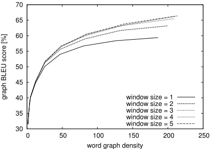
In Figure 4, we show the graph BLEU scores for the IWSLT task. We observe that, similar to the GPER, the GBLEU score increases significantly al-ready for small word graph densities. We attribute this to the fact that the BLEU score and especially the PER are less affected by errors of the word or-der than the WER. This also indicates that produc-ing translations with correct word order, i.e. syntac-tically well-formed sentences, is one of the major problems of current statistical machine translation systems.
6 Conclusion
30 35 40 45 50 55 60 65 70
0 50 100 150 200 250
graph BLEU score [%]
[image:8.612.75.293.59.213.2]word graph density window size = 1 window size = 2 window size = 3 window size = 4 window size = 5
Figure 4: IWSLT Chinese–English: Graph BLEU score as a function of the word graph density.
pruning method for word graphs. Using these tech-nique, we have generated compact word graphs for two Chinese–English tasks. For the IWSLT task, the graph error rate drops from about 50% for the single-best hypotheses to 17% of the word graph. Even for the NIST task, with its very large vocabulary and long sentences, we were able to reduce the graph er-ror rate significantly from about 64% down to 23%.
Acknowledgment
This work was partly funded by the European Union under the integrated project TC-Star (Technology and Corpora for Speech to Speech Translation, IST-2002-FP6-506738, http://www.tc-star.org).
References
Y. Akiba, M. Federico, N. Kando, H. Nakaiwa, M. Paul, and J. Tsujii. 2004. Overview of the IWSLT04 evaluation cam-paign. InProc. of the Int. Workshop on Spoken Language Translation (IWSLT), pages 1–12, Kyoto, Japan, Septem-ber/October.
S. Bangalore and G. Riccardi. 2001. A finite-state approach to machine translation. InProc. Conf. of the North American Association of Computational Linguistics (NAACL), Pitts-burgh, May.
S. Kanthak, D. Vilar, E. Matusov, R. Zens, and H. Ney. 2005. Novel reordering approaches in phrase-based statistical ma-chine translation. In43rd Annual Meeting of the Assoc. for Computational Linguistics: Proc. Workshop on Building and Using Parallel Texts: Data-Driven Machine Translation and Beyond, Ann Arbor, MI, June.
K. Knight and Y. Al-Onaizan. 1998. Translation with finite-state devices. In D. Farwell, L. Gerber, and E. H. Hovy,
editors,AMTA, volume 1529 ofLecture Notes in Computer Science, pages 421–437. Springer Verlag.
S. Kumar and W. Byrne. 2003. A weighted finite state trans-ducer implementation of the alignment template model for statistical machine translation. InProc. of the Human Lan-guage Technology Conf. (HLT-NAACL), pages 63–70, Ed-monton, Canada, May/June.
L. Mangu, E. Brill, and A. Stolcke. 2000. Finding consensus in speech recognition: Word error minimization and other applications of confusion networks. Computer, Speech and Language, 14(4):373–400, October.
M. Mohri and M. Riley. 2002. An efficient algorithm for the n-best-strings problem. InProc. of the 7th Int. Conf. on Spoken Language Processing (ICSLP’02), pages 1313–1316, Den-ver, CO, September.
F. J. Och and H. Ney. 2002. Discriminative training and max-imum entropy models for statistical machine translation. In
Proc. of the 40th Annual Meeting of the Association for Com-putational Linguistics (ACL), pages 295–302, Philadelphia, PA, July.
F. J. Och, R. Zens, and H. Ney. 2003. Efficient search for in-teractive statistical machine translation. InEACL03: 10th Conf. of the Europ. Chapter of the Association for Com-putational Linguistics, pages 387–393, Budapest, Hungary, April.
F. J. Och. 2003. Minimum error rate training in statistical ma-chine translation. In Proc. of the 41th Annual Meeting of the Association for Computational Linguistics (ACL), pages 160–167, Sapporo, Japan, July.
N. Ueffing and H. Ney. 2004. Bayes decision rule and confidence measures for statistical machine translation. In
Proc. EsTAL - Espa˜na for Natural Language Processing, pages 70–81, Alicante, Spain, October.
N. Ueffing, F. J. Och, and H. Ney. 2002. Generation of word graphs in statistical machine translation. In Proc. of the Conf. on Empirical Methods for Natural Language Process-ing (EMNLP), pages 156–163, Philadelphia, PA, July.
R. Zens and H. Ney. 2004. Improvements in phrase-based statistical machine translation. In Proc. of the Human Language Technology Conf. (HLT-NAACL), pages 257–264, Boston, MA, May.